Background gamma rhythmicity and attention in cortical local circuits: A computational study

Models of Gamma Rhythms

We first summarize some pertinent facts about models of gamma rhythms in networks of E- and I-cells (excitatory and inhibitory cells) (see ref. 30 for a review).

Interneuronal Network Gamma (ING). Gamma oscillations in the CA1 region of the hippocampus can be induced in vitro by the application of muscarinic agonists, even during the blockade of ionotropic excitatory postsynaptic potentials (31). This type of gamma rhythm, called ING (30), does not depend on the participation of E-cells, and individual I-cells fire at or near gamma frequency. ING has been simulated in large-scale, biophysically realistic computational models (see, e.g., ref. 32 for references). It has also been simulated and analyzed in minimal network models, with the aim of understanding the dynamical mechanisms that generate the observed network behavior. Modeling of the latter kind (33–37) has clarified the basic dynamical properties of ING coherence. Wang and Buzsáki (36) and White et al. (37) have shown that ING is fragile, in the sense that coherence is usually lost when a modest amount of heterogeneity in the drives to the I-cells is introduced. Tiesinga and José (35) have described a more robust ING-like rhythm in which there are stochastic fluctuations in the drive to the I-cells, and individual I-cells do not participate on every population cycle. Although E-cells are not needed for ING, a population of E-cells may be entrained by a population of I-cells firing rhythmically and in synchrony (31).

Pyramidal-Interneuronal Network Gamma (PING). Gamma oscillations in hippocampal slices can also be induced by tetanic stimulation (38). In this form of gamma, called PING (30), individual E-cells fire at or near gamma frequency, and their active participation is crucial: The E-cells drive and synchronize the I-cells, and the I-cells gate and synchronize the E-cells. Biophysically detailed simulations of PING were presented in ref. 39 and motivated our own recent minimal-network models of PING (40, 41). In ref. 40, we studied how variations in external drives can create or abolish PING rhythms. If drive to the I-cells becomes too strong or if drive to the E-cells becomes too weak, the PING mechanism fails: Either the I-cells synchronize at too high a frequency to be entrained by the E-cells (phase walk-through) or the I-cells do not synchronize, and their activity leads to the suppression of the E-cells, thereby removing the mechanism that could create a synchronous rhythm. In the parameter regime in which phase walkthrough occurs, no PING rhythm is possible. However, there is a region of bistability in parameter space within which both suppression of the E-cells by asynchronous activity of the I-cells and PING are possible (see figure 7C of ref. 40).

Weak Gamma. In another type of gamma rhythm, the E-cells spike irregularly and at a mean frequency much below that of the population rhythm. The persistent hippocampal and neocortical gamma oscillations described above are of this type. We call such gamma rhythms “weak,” and sometimes use the word “strong” to characterize gamma rhythms in which E-cells participate more frequently. Several varieties of weak gamma are theoretically possible (see Model Networks). We shall consider here only one of them, a PING-like rhythm in which the E-cells receive randomly fluctuating drive and gamma-frequency oscillations are generated by the following mechanism: Synaptic inhibition from a population spike of the I-cells abruptly halts spiking of the E-cells. As the inhibition decays, the most depolarized of the stochastically driven E-cells begin to reach threshold and spike again. The resulting volley of E-cell spikes quickly triggers a new I-cell population spike, which again halts E-cell spiking, initiating the next cycle.

A biophysically detailed computational model of such a rhythm was described by Traub et al. (32). In their model, there is a source of noisy spiking activity in the axonal compartments of the model pyramidal cells generated by ectopic axonal spiking and amplified by axo-axonal gap junctions (42). Brunel and Wang (43) have investigated a simplified model of such a network composed of integrate-and-fire neurons.

Methods

Model Neurons. The neuronal model used in this article is that of Ermentrout and Kopell (44), a one-compartment reduction of the model of Traub and Miles (45). The basic structure of the model is the same for both E- and I-cells. In the absence of synaptic currents, the equation governing the membrane potential V takes the form of the classical Hodgkin–Huxley equation (46):

[1]

Here, m = m_∞(V) = a_m(V)/[a_m(V) + b_m(V)] with a_m(V) = 0.32(54 + V)/{1 – exp[–0.25(V + 54)]} and b_m(V) = 0.28(27 + V)/{exp[0.2(V + 27)] – 1}, h = max(1 – 1.25n, 0), and the equation for n is dn/dt = a_n(V)(1 – n) – b_n(V)n with a_n(V) = 0.032(52 + V)/{1 – exp[–0.2(V + 52)]} and b_n(V) = 0.5 exp[–0.025(57 + V)]. The letters C, V, t, g, and I denote capacitance density, voltage, time, conductance density, and current density, respectively. The units used for these quantities are μF/cm², ms, mV, mS/cm², and μA/cm², respectively. For brevity, units will often be omitted from here on. The parameter values of the model are C = 1, g_Na = 100, V_Na = 50, g_K = 80, V_K = –100, g_L = 0.1, and V_L = –67.

To represent slow hyperpolarizing currents in the E-cells activated by depolarization, e.g., an M current, we adopt the model of Olufsen et al. (47), a slight variation on the model of Crook et al. (48); the term g_Mw(V_K – V) is added to the right-hand side of Eq. 1, with dw/dt = [w_∞(V) – w]/τ_M(V), w_∞(V) = 1/{1 + exp[–(V + 35)/10]}, and τ_M(V) = 400/{3.3 exp[(V + 35)/20] + exp[–(V + 35)/20]}.

Model Synapses. We consider networks of N_E E-cells and N_I I-cells. We assume that synaptic connectivity is all-to-all, modeling synaptic connections mediated by NMDA receptors (E → E), AMPA (α-amino-3-hydroxy-5-methyl-4-isoxazolepropionic acid) receptors (E → E and E → I), and GABA_A receptors (I → E and I → I). GABA_A synapses are modeled by a term of the form (g/N_I)Σs_ij(t) (V_I – V_j) on the right-hand side of the equation governing the membrane potential of cell j, where V_I = –80, g = g_IE if cell j is excitatory, g = g_II if cell j is inhibitory, and the sum extends over the indices i of the I-cells. The gating variables s = s_ij satisfy

[2]

with τ_R = 0.5, τ_D = 10, and V_pre equal to the membrane potential of the presynaptic (ith) cell. This models inhibition from fast-spiking interneurons, believed to be important for the production of gamma rhythms. The term (1 + tanh(V_pre/10))/2 can be thought of as a normalized neurotransmitter concentration, nearly equivalent to equation 5.5 of ref. 49. Following Ermentrout and Kopell (44), we have rewritten the equation in terms of the hyperbolic tangent and made the very minor, aesthetically motivated approximation of setting the half-activation voltage to 0 mV (in ref. 49, the half-activation voltage is 2 mV). Similarly, AMPA synapses are modeled by a term of the form (g/N_E)Σs_ij(t) (V_E – V_j) on the right-hand side of the equation governing the membrane potential of cell j, where V_E = 0, g = g_EE,AMPA if cell j is excitatory, g = g_EI if cell j is inhibitory, and the sum extends over the indices i of the E-cells. The s_ij satisfy Eq. 2, with τ_R = 0.2 and τ_D = 2. NMDA-receptor-mediated E → E synapses are modeled similarly, with g = g_EE,NMDA. In modeling the magnesium block of NMDA receptor channels, we follow Jahr and Stevens (50, 51), assuming an external magnesium concentration of 1 mM:

with τ_R = 1, τ_D = 100, and V_post equal to the membrane potential of the postsynaptic (jth) cell.

Model Networks. All simulation results shown in this article are for N_E = 160 E-cells and N_I = 40 I-cells. However, results for larger or (somewhat) smaller networks are quite similar if the synaptic strengths are scaled by N_E and N_I, as described under Model Synapses. Synaptic connectivity is all-to-all, except for E → E synapses, as described below. Each E-cell receives a baseline current input, I_E, that is constant in time. The value of I_E is chosen at random and uniformly distributed in an interval [, ]. In addition, each E-cell receives an independent Poisson stream of excitatory postsynaptic potentials (EPSPs) with a mean frequency . 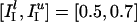The associated synaptic conductance jumps to a maximal value instantaneously when the presynaptic spike arrives, then decays exponentially, with a time constant of 2 ms. Similarly, the I-cells are driven by a constant current input, I_I, chosen at random with uniform distribution in [, ] and independent Poisson streams of EPSPs with maximal conductance and mean frequency . Over a wide range of parameter values, such networks generate a PING-like weak gamma rhythm, which we will refer to as “weak PING.”

We note that there are alternative ways of generating weak gamma rhythms. One possibility is an ING rhythm, with entrained E-cells receiving randomly fluctuating external drive. Such rhythms can be fragile to heterogeneity and noise (but see ref. 35). We have chosen a PING-like model rhythm here because it appears that carbachol-induced gamma rhythms in vitro are PING-like and not ING-like (see Discussion). Another possibility is a network in which the E-cells receive randomly fluctuating inhibitory input from the I-cells, rather than randomly fluctuating external input; this can be accomplished by giving the I-cells noisy external drive and making the I → E connection sparse and random. However, our experience indicates that, for rhythms of this kind, the mean spiking frequency of the E-cells is highly sensitive to changes in the strengths of the I → E synapses. Analysis of an idealized network (not presented here) confirms and explains this conclusion.

Numerics. We solve the differential equations using the midpoint method with Δt = 0.01 ms. All simulations are initialized asynchronously in the following sense. Model neurons driven above their spiking threshold are initialized at a random point on their limit cycle, chosen so that the time to the first spike, in the absence of any synaptic inputs, would be uT, where T is the intrinsic period of the neuron and u ∈ [0, 1] is random, with uniform distribution. Model neurons driven below their spiking threshold are initialized at their (uniquely determined) stable fixed points.

Results

Background Gamma Rhythm. Fig. 1a shows spike rastergrams obtained from a simulation of 160 E-cells and 40 I-cells with 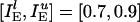; ; ; ; ; g_EI = 1.0; g_IE = 0.5; g_II = 0.1; and g_EE,AMPA = g_EE,NMDA = g_M = 0. The I-cells synchronize and spike regularly at ≈37 Hz. Individual E-cells spike irregularly and infrequently, at an average frequency of ≈3.5 Hz.

Adaptation Currents Weaken Activity of the E-Cells and, in Turn, Reduce or Abolish Coherence of the I-Cells. When an adaptation current with g_M = 0.1 is added to the E-cells, they are largely suppressed, and the I-cells lose coherence (see Fig. 1b). The frequency of the I-cells is ≈28 Hz in Fig. 1b. The transition from rhythmicity to arhythmicity and suppression of the E-cells is rapid as g_M is increased; for instance, a clean rhythm, quite similar to that of Fig. 1a, is still obtained when g_M = 0.05 (data not shown). This transition is similar to crossing the “suppression boundary,” as described in ref. 40. (The two are not the same, because raising g_M is not equivalent to lowering the external drive to the E-cells.)

Loss of Coherence Contributes to Suppression of E-Cells. In the simulation of Fig. 1b, the E-cells are suppressed for two reasons. First, adaptation currents make E-cells less excitable. Second, the I-cell population is more effective when it spikes asynchronously than it is when it spikes in synchrony (see appendix A of ref. 40). To demonstrate the importance of the loss of coherence by itself, we show in Fig. 1c the results of a simulation in which there are no adaptation currents, but spiking of the I-cells has been made less coherent by setting g_II = 0. (As discussed in detail in ref. 40, I → I synapses often stabilize PING rhythms, even though they are not, in principle, necessary for PING.) In Fig. 1c, the mean spiking frequency of the I-cells is 33 Hz, less than the population frequency in Fig. 1a. However, the reduced coherence of the I-cell firing makes inhibition so powerful that the E-cells are almost entirely suppressed.

Specific Excitation Leads to Specific Strong PING. Next, we present the results of simulations in which extra external drive was given to a subset D of the E-cells. We think, here, of a cell ensemble made more excitable as a result of either sensory input or selective “top-down” excitation. In our experiments, we take D to be the set of E-cells 11–30; because there is no spatial structure in our networks, we could equally well have chosen any other set of 20 E-cells. Fig. 2a shows the results of a simulation like that of Fig. 1a but with the external drive to the cells in D increased by 0.5. With the increased excitatory drive, the population frequency rises slightly (see ref. 40), from 37 Hz in Fig. 1a to ≈39 Hz. The E-cells in D participate frequently but not on every cycle; their mean spiking frequency is ≈23 Hz. The mean frequency of the remaining E-cells is reduced to ≈2 Hz, from ≈3.5 Hz in Fig. 1a.

Adaptation Currents and Loss of Coherence Weaken Response to Specific Excitation. Fig. 2b shows the result of a simulation similar to that underlying Fig. 2a but with g_M raised from 0 to 0.2. The activity of the E-cells is weakened considerably. In Fig. 2b, the mean spiking frequency of the I-cells is 30 Hz, lower than the 39 Hz seen in Fig. 2a. Nevertheless, the mean spiking frequency of the E-cells in D has been reduced from 23 Hz to 4.5 Hz.

Adaptation currents lower activity in the E-cells directly, by making the E-cells less excitable, but also indirectly, by reducing coherence of the I-cell population and thereby making inhibition more powerful. We present a simulation demonstrating the importance of the loss of coherence alone to the effectiveness of specific excitation. In the simulation of Fig. 2a, we set g_II = 0 and raise to 0.1 but introduce no adaptation currents: g_M = 0. The result is displayed in Fig. 2c. The rhythm in the I-cells is lost. The loss of rhythm, by itself, greatly weakens response to the specific excitation. The mean spiking frequency of the I-cells is 38 Hz, slightly lower than the 39 Hz of Fig. 2a; however, the spiking frequency of the cells in D is only ≈7 Hz, much lower than the 23 Hz of Fig. 2a.

Fig. 2d illustrates the point in yet another way. The parameter values in Fig. 2d are ; ; ; ; ; g_EI = 1.0; g_IE = 0.8; g_II = 0.3; and g_EE,AMPA = g_EE,NMDA = g_M = 0. These parameters are chosen such that intervals of rhythmicity and arhythmicity alternate intermittently. When, by chance, there is a brief surge in the activity of the I-cells, the E-cells are partially suppressed, thus abolishing the rhythm. A random drop in the firing frequency of the I-cells allows the E-cells to recover and fire a nearly synchronous population spike, which restores the rhythm. Intervals of arhythmicity coincide with intervals of low firing in D. This behavior is strongly reminiscent of the parameter regime described in ref. 40, in which both PING and suppression of the E-cells by asynchronous activity of the I-cells are stable network states. In the simulation of Fig. 2d, random events give rise to toggling between the two states.

Acceleration of the Inhibitory Population Rhythm Is a Mechanism for Suppressing Distractors. We now consider a second subset of the E-cells, denoted by L, that is excited more strongly than the cells in D. In this context, we think of D as a distractor. We take L to encompass E-cells 121–140. For now, we let D consist of E-cells 11–30, as before; later, we will also consider a case in which L and D overlap. Fig. 3a shows the results of a simulation similar to that of Fig. 2a, with the external drive to the cells of D raised by 0.5, as in Fig. 2a, but also with the external drive to the cells of L raised by 0.7. Activity in D is now largely suppressed; the mean spiking frequency in D is 10 Hz (down from 23 Hz in Fig. 2a), whereas in L, it is 30 Hz. The suppression of D is accomplished by a very slight acceleration of the population rhythm of the I-cells, from 39 Hz in Fig. 2a to 41 Hz in Fig. 3a. The more rapid spiking of the I-cell population suppresses the cells of D; this mechanism will be discussed further below. Note that the suppression of D is instantaneous.

Recurrent Excitation Facilitates Suppression of Distractors. In Fig. 3b, we show the results of a simulation similar to that of Fig. 3a, with NMDA-receptor-mediated synapses added within L and D (g_EE,NMDA = 1.0) but not elsewhere. The recurrent excitation adds drive to both assemblies. However, because the cells in L spike more than those in D in the absence of any recurrent excitation (Fig. 3a), L gains more drive than D when the E → E synapses are introduced. This effect is amplified by the dependence of NMDA receptors on postsynaptic voltage and enhances the suppression of D by L; the mean frequency of cells in L is 39 Hz in Fig. 3b (up from 30 Hz in Fig. 3a), and the mean frequency of cells in D is 7 Hz (down from 10 Hz); the population rhythm is slightly accelerated, to 43 Hz (from 41 Hz). Note, again, that the suppression of D is instantaneous.

Fig. 3 c and d illustrates the same point for overlapping competing assemblies. Here, we have redefined D as the set of E-cells 107–126; thus, the intersection L \ D consists of cells 121–125. The boundaries of L are indicated by solid horizontal lines in Fig. 3 c and d and those of D by dash–dot lines. Fig. 3c shows the results of a simulation without any E → E synapses. The cells in L spike much more frequently than those outside L. However, the cells in L \ D (cells belonging to L but not to D) spike less frequently than those in the overlap L \ D. Participation of the cells in L \ D improves greatly when E → E synapses (g_EE,AMPA = 0.3 and g_EE,NMDA = 1.0) are added within L and D (see Fig. 3d).

Gamma Oscillations Facilitate Suppression of Distractors. We will argue that the suppression of D by L is more effective in the presence of a rhythm than in its absence. We begin with a heuristic argument. In the presence of a rhythm, for instance, in the simulation of Fig. 3a, population spikes of L trigger population spikes of I-cells. When the I-cells spike, the cells of L have just spiked and are therefore least susceptible to inhibition, whereas the cells of D are close to spiking and are therefore most susceptible to inhibition. Thus, the timing of the inhibition favors L. One might think of the following simplified version of the mechanism. Disregard all noise and suppose that the population spikes of L were perfectly synchronous, that they triggered the inhibitory population spikes without any delay, and that the inhibitory population spikes instantaneously reset all E-cells to the same point, P, in phase space. Clearly, no E-cell with below-maximal external drive could ever spike under those assumptions. Furthermore, if E-cells reset to the same point P after spiking, the inhibition would not affect the cells in L at all. Note that the conclusion that no E-cell with below-maximal external drive could ever spike does not require the unrealistic assumption that inhibition causes instantaneous reset of all E-cells. One needs only the assumption that the spiking of the E-cells after an inhibitory population spike is timed as if they had all been reset to the same point in phase space. This assumption is more realistic (see figure 5C of ref. 41).

By contrast, if L recruited asynchronous inhibition to suppress D, this inhibition would strongly affect L itself, especially if L were only slightly more excited than D. To illustrate this effect, we show, in Fig. 3e, the results of a simulation with parameters ; ; ; ; ; ; g_EI = 0; g_IE = 0.5; g_II = 0; and g_EE,AMPA = g_EE,NMDA = g_M = 0. The tonic drive to the I-cells has been entirely replaced by frequent, strong random synaptic input here, and all network-internal synapses except the I → E synapses have been removed. The I-cells spike asynchronously in this simulation. The frequency of the synaptic input to the I-cells has been chosen to bring the mean frequency of the cells in D to 7 Hz, the same value as in Fig. 3b. The mean frequency of the cells in L is now 20 Hz, much lower than the 39 Hz of Fig. 3b. Thus, if L suppressed D by recruiting asynchronous inhibition (by a mechanism not modeled here) to bring the cells of D down to a mean frequency of 7 Hz, the result would be a significant slowdown in activity within L itself.

We use two reduced networks to further illustrate this point. First, we consider a network of three cells: two E-cells, called “L” and “D,” analogous to our earlier notation, and a single I-cell, reflecting the assumption of synchronization of the I-cell population. We assume that the two E-cells receive tonic, deterministic drive only and denote their intrinsic frequencies by f_L and f_D. The I-cell is driven at I_I = 0. We introduce E → I synapses with g_EI = 0.9; i.e., the maximal conductance associated with each of the two E → I synapses is 0.9/2 = 0.45. This value is chosen so that a spike of one of the E-cells triggers a spike of the I-cell rapidly (within <1 ms), but the I-cell does not fire spike doublets. We further introduce I → E synapses, with maximal conductance set precisely large enough to suppress D but not larger. For simplicity, we omit E → E and I → I synapses and adaptation currents. We denote the frequency of L in the network by ; the superscript r stands for “rhythmic.” The circles connected by solid line segments in Fig. 4 show as a function of f_D, with f_L = 75 fixed. In all cases, , reflecting that the price of suppression of D is a slowdown of L. For values of f_D close to f_L, suppression of D is difficult and requires , i.e., suppression of D requires substantial slowdown of L.

We compare this network with a second comprising only two uncoupled E-cells, L and D, subject to common, constant synaptic inhibition; this is an idealization of input from a large population of asynchronously spiking I-cells. As before, the E-cells have intrinsic frequencies f_L and f_D, resulting from tonic, deterministic external drives, and the strength of synaptic inhibition is set precisely large enough to suppress D but not larger. We denote the frequency of L in this network by ; the superscript a stands for “asynchronous.” The squares connected by dashed line segments in Fig. 4 show as a function of _fD, again, with f_L = 75 fixed. In all cases, . Thus, the cost of suppressing D, measured by the required slowdown of L, is greater when inhibition is asynchronous than when inhibition is rhythmic. This effect is particularly significant when f_D is close to f_L = 75.

Discussion

We have proposed a model linking cholinergic modulation of adaptation currents, gamma rhythms, and attention and illustrated its properties in simulations of a generic E/I network that was originally devised as a minimal model of persistent gamma oscillations in vitro (17, 18, 21, 32). Specifically, we have shown that reducing adaptation currents can change the state of the network from asynchrony to weak gamma rhythmicity; that such emergent coherence in the spiking of the interneurons enhances input sensitivity; that specific input induces specific patterns of strong gamma oscillations superimposed on a weak gamma background; and that gamma oscillations enhance the suppression of less strongly excited neuronal ensembles (distractors) by more strongly excited ones.

Several of the components of our model have appeared, in various forms, in previous work. Below, we briefly discuss some of this work in relation to this study.

The transition we have described from asynchrony to weak PING depends on an increase in pyramidal cell excitability resulting from cholinergic modulation. Tiesinga et al. (52) have shown that transitions to gamma oscillation may also result from raising interneuron excitability. In our simulations, the I-cells are sufficiently depolarized that a further increase in their excitability would lead to ING. However, fast glutamatergic transmission is known to be required for the generation of carbachol-induced persistent gamma rhythms in slice preparations of hippocampus (17) and somatosensory cortex (18), suggesting that such rhythms are PING-like. We note, also, that gamma oscillations induced by carbachol in vitro (17, 18) or facilitated by cholinergic modulation in vivo (16) are significantly reduced by muscarinic antagonists, suggesting that the most important effects of acetylcholine in the generation of these rhythms are mediated by muscarinic receptors.

Tiesinga et al. (53, 54) found that increased coherence in the spiking of interneurons leads to increased input sensitivity and suggested synchronization of interneuron networks as a mechanism for attentional gain modulation. Similarly, Lumer (55) observed that “effective connectivity, of an inhibitory nature, is decreased in the context of synchronization.” For a related analysis, see Börgers and Kopell (appendix A, theorem 2 of ref. 40).

Fast suppression mechanisms based on oscillatory network dynamics have been studied in networks exhibiting (strong) PING by Olufsen et al. (47), in interneuron networks by Tiesinga and Sejnowski (56), and in more abstract form by Jin and Seung (57) and Wang and Slotine (58, 59). Lumer (55) found that synchronization disrupts competition in an E/I spiking network. However, in his model, the competing ensembles were in precise synchrony; in our model, the suppression of one ensemble by another relies on the fact that the cells in D are not quite ready to spike when those in L spike. A different model of stimulus competition based on the timing of inhibition, involving the interaction of two pools of interneurons, has also been proposed by Tiesinga (60).

It has been suggested (see, e.g., refs. 11 and 61) that rate and synchrony might represent independent channels, such that stimulus properties are rate-coded, whereas attention is encoded by synchrony. In the model presented here, however, attentional state is signaled by changes in both rate and synchrony: The cells of selected ensembles spike at higher rates than unselected cells, and their downstream impact is further enhanced by the synchrony of their firing (see, e.g., refs. 62 and 63). Spiking in unselected cells is also entrained to the population rhythm, but it is the selected cells, firing more frequently and synchronizing more precisely, that dominate the output of the local circuit.

Our generic E/I network is a highly idealized caricature of a local circuit in the superficial layers of a single cortical column; connectivity is all-to-all, conduction delays are neglected, and we have modeled only one of the several effects of acetylcholine release in neocortex (although we believe it is the effect most important for generating the weak gamma rhythm). Larger and less schematic models will likely be needed to address specific experimental data (e.g., refs. 9, 64, and 65). Nevertheless, this work demonstrates, in principle, how a cortical network supporting weak gamma oscillations can implement computations that are widely believed to underlie preparatory and selective attention.

References

- 1.Gruber, T., Müller, M. M., Keil, A. & Elbert, T. (1999) Clin. Neurophysiol. 110, 2074–2085. [DOI] [PubMed] [Google Scholar]
- 2.Herrmann, C. S. & Mecklinger, A. (2001) Visual Cognit. 8, 593–608. [Google Scholar]
- 3.Maloney, K. J., Cape, E. G., Gotman, J. & Jones, B. E. (1996) Neuroscience 76, 541–555. [DOI] [PubMed] [Google Scholar]
- 4.Tallon-Baudry, C., Bertrand, O., Peronnet, C. F. & Pernier, J. (1997) J. Neurosci. 17, 722–734. [DOI] [PMC free article] [PubMed] [Google Scholar]
- 5.Tiitinen, H., May, P. & Näätänen, R. (1997) Prog. Neuropsychopharmacol. Biol. Psychiatry 21, 751–771. [DOI] [PubMed] [Google Scholar]
- 6.Chrobak, J. J. & Buzsáki, G. (1998) J. Neurosci. 18, 388–398. [DOI] [PMC free article] [PubMed] [Google Scholar]
- 7.Engel, A. K., Fries, P. & Singer, W. (2001) Nat. Rev. Neurosci. 2, 704–716. [DOI] [PubMed] [Google Scholar]
- 8.Fell, J., Fernández, G., Klaver, P., Elger, C. E. & Fries, P. (2003) Brain Res. Rev. 42, 265–272. [DOI] [PubMed] [Google Scholar]
- 9.Fries, P., Reynolds, J. H., Rorie, A. E. & Desimone, R. (2001) Science 291, 1560–1563. [DOI] [PubMed] [Google Scholar]
- 10.Liang, H., Bressler, S. L., Ding, M., Desimone, R. & Fries, P. (2003) Neurocomputing 52–54, 481–487.12934604 [Google Scholar]
- 11.Niebur, E. (2002) Biosystems 67, 157–166.12459295 [Google Scholar]
- 12.Steinmetz, P. N., Roy, A., Fitzgerald, P. J., Hsiao, S. S., Johnson, K. O. & Niebur, E. (2000) Nature 404, 187–190. [DOI] [PubMed] [Google Scholar]
- 13.Sarter, M., Givens, B. & Bruno, J. P. (2001) Brain Res. Rev. 35, 146–160. [DOI] [PubMed] [Google Scholar]
- 14.Cape, E. G. & Jones, B. E. (1998) J. Neurosci. 18, 2653–2666. [DOI] [PMC free article] [PubMed] [Google Scholar]
- 15.Dringenberg, H. C. & Vanderwolf, C. H. (1997) Exp. Brain Res. 116, 160–174. [DOI] [PubMed] [Google Scholar]
- 16.Rodriguez, R., Kallenbach, U., Singer, W. & Munk, M. H. J. (2004) J. Neurosci. 24, 10369–10378. [DOI] [PMC free article] [PubMed] [Google Scholar]
- 17.Fisahn, A., Pike, F. G., Buhl, E. H. & Paulsen, O. (1998) Nature 394, 186–189. [DOI] [PubMed] [Google Scholar]
- 18.Buhl, E. H., Tamás, G. & Fisahn, A. (1998) J. Physiol. (London) 513, 117–126. [DOI] [PMC free article] [PubMed] [Google Scholar]
- 19.Barkai, E. & Hasselmo, M. (1994) J. Neurophysiol. 72, 644–658. [DOI] [PubMed] [Google Scholar]
- 20.Hasselmo, M. E. (1999) Trends Cognit. Sci. 3, 351–359. [DOI] [PubMed] [Google Scholar]
- 21.Dickson, C. T., Biella, G. & deCurtis, M. (2000) J. Neurosci. 20, 7846–7854. [DOI] [PMC free article] [PubMed] [Google Scholar]
- 22.Cunningham, M. O., Davies, C. H., Buhl, E. H., Kopell, N. & Whittington, M. A. (2003) J. Neurosci. 23, 9761–9769. [DOI] [PMC free article] [PubMed] [Google Scholar]
- 23.Parasuraman, R., Warm, J. & See, J. (1998) in The Attentive Brain, ed. Parasuraman, R. (MIT Press, Cambridge, MA), pp. 221–256.
- 24.Kay, L. M. (2003) J. Integr. Neurosci. 2, 31–44. [DOI] [PubMed] [Google Scholar]
- 25.Linkenkaer-Hansen, K., Nikulin, V., Palva, S., Ilmoniemi, R. & Palva, J. (2004) J. Neurosci. 24, 10186–10190. [DOI] [PMC free article] [PubMed] [Google Scholar]
- 26.Desimone, R. (1998) Philos. Trans. R. Soc. London B 353, 1245–1255. [DOI] [PMC free article] [PubMed] [Google Scholar]
- 27.Itti, L. & Koch, C. (2001) Nat. Rev. Neurosci. 2, 194–203. [DOI] [PubMed] [Google Scholar]
- 28.Kastner, S. & Ungerleider, L. (2001) Neuropsychologia 39, 1263–1276. [DOI] [PubMed] [Google Scholar]
- 29.Reynolds, J. & Chelazzi, L. (2004) Annu. Rev. Neurosci. 27, 611–647. [DOI] [PubMed] [Google Scholar]
- 30.Whittington, M. A., Traub, R. D., Kopell, N., Ermentrout, B. & Buhl, E. H. (2000) Int. J. Psychophysiol. 38, 315–336. [DOI] [PubMed] [Google Scholar]
- 31.Whittington, M. A., Traub, R. D. & Jefferys, J. G. R. (1995) Nature 373, 612–615. [DOI] [PubMed] [Google Scholar]
- 32.Traub, R. D., Bibbig, A., Fisahn, A., LeBeau, F. E. N., Whittington, M. A. & Buhl, E. H. (2000) Eur. J. Neurosci. 12, 4093–4106. [DOI] [PubMed] [Google Scholar]
- 33.Chow, C. C., White, J. A., Ritt, J. & Kopell, N. (1998) J. Comp. Neurosci. 5, 407–420. [DOI] [PubMed] [Google Scholar]
- 34.Lytton, W. & Sejnowski, T. J. (1991) J. Neurophysiol. 66, 1059–1097. [DOI] [PubMed] [Google Scholar]
- 35.Tiesinga, P. H. E. & José, J. V. (2000) Network Comput. Neural Syst. 11, 1–23. [PubMed] [Google Scholar]
- 36.Wang, X.-J. & Buzsáki, G. (1996) J. Neurosci. 16, 6402–6413. [DOI] [PMC free article] [PubMed] [Google Scholar]
- 37.White, J., Chow, C., Ritt, J., Soto-Trevino, C. & Kopell, N. (1998) J. Comput. Neurosci. 5, 5–16. [DOI] [PubMed] [Google Scholar]
- 38.Whittington, M. A., Stanford, I. M., Colling, S. B., Jefferys, J. G. R. & Traub, R. D. (1997) J. Physiol. (London) 502, 591–607. [DOI] [PMC free article] [PubMed] [Google Scholar]
- 39.Traub, R. D., Jefferys, J. G. R. & Whittington, M. (1997) J. Comput. Neurosci. 4, 141–150. [DOI] [PubMed] [Google Scholar]
- 40.Börgers, C. & Kopell, N. (2005) Neural Comput. 17, 557–608. [DOI] [PubMed] [Google Scholar]
- 41.Börgers, C. & Kopell, N. (2003) Neural Comput. 15, 509–539. [DOI] [PubMed] [Google Scholar]
- 42.Schmitz, D., Schuchmann, S., Fisahn, A., Draguhn, A., Buhl, E. H., Petrasch-Parwez, E., Dermietzel, R., Heinemann, U. & Traub, R. D. (2001) Neuron 31, 669–671. [DOI] [PubMed] [Google Scholar]
- 43.Brunel, N. & Wang, X.-J. (2003) J. Neurophysiol. 90, 415–430. [DOI] [PubMed] [Google Scholar]
- 44.Ermentrout, G. B. & Kopell, N. (1998) Proc. Natl. Acad. Sci. USA 95, 1259–1264. [DOI] [PMC free article] [PubMed] [Google Scholar]
- 45.Traub, R. D. & Miles, R. (1991) Neuronal Networks of the Hippocampus (Cambridge Univ. Press, Cambridge, U.K.).
- 46.Hodgkin, A. L. & Huxley, A. F. (1952) J. Physiol. (London) 117, 500–544. [DOI] [PMC free article] [PubMed] [Google Scholar]
- 47.Olufsen, M., Whittington, M. A., Camperi, M. & Kopell, N. (2003) J. Comput. Neurosci. 14, 33–54. [DOI] [PubMed] [Google Scholar]
- 48.Crook, S. M., Ermentrout, G. B. & Bower, J. M. (1998) Neural Comput. 10, 837–854. [DOI] [PubMed] [Google Scholar]
- 49.Destexhe, A. & Sejnowski, T. J. (2001) Thalamocortical Assemblies (Oxford Univ. Press, New York).
- 50.Jahr, C. E. & Stevens, C. F. (1990) J. Neurosci. 10, 1830–1837. [DOI] [PMC free article] [PubMed] [Google Scholar]
- 51.Jahr, C. E. & Stevens, C. F. (1990) J. Neurosci. 10, 3178–3182. [DOI] [PMC free article] [PubMed] [Google Scholar]
- 52.Tiesinga, P. H. E., Fellous, J.-M., José, J. V. & Sejnowski, T. J. (2001) Hippocampus 11, 251–274. [DOI] [PubMed] [Google Scholar]
- 53.Tiesinga, P. H. E., Fellous, J.-M., Salinas, E., José, J. V. & Sejnowski, T. J. (2004) Neurocomputing 58–60, 641–646. [DOI] [PMC free article] [PubMed] [Google Scholar]
- 54.Tiesinga, P. H. E. (2002) in Developments in Mathematical and Experimental Physics (Vol. B), eds. Macias, A., Uribe, F. J. & Diaz, E. (Kluwer, Boston), pp. 99–112.
- 55.Lumer, E. D. (2000) Neural Comput. 12, 181–194. [DOI] [PubMed] [Google Scholar]
- 56.Tiesinga, P. H. E. & Sejnowski, T. J. (2004) Neural Comput. 16, 251–275. [DOI] [PMC free article] [PubMed] [Google Scholar]
- 57.Jin, D. Z. & Seung, H. S. (2002) Phys. Rev. E Stat. Phys. Plasmas Fluids Relat. Interdiscip. Top. 65, 051922. [Google Scholar]
- 58.Wang, W. & Slotine, J.-J. E. (2003) arXiv:q-bio.NC/0312025.
- 59.Wang, W. & Slotine, J.-J. E. (2003) arXiv:q-bio.NC/0401001.
- 60.Tiesinga, P. H. E. (2004) arXiv:q-bio.NC/0410019.
- 61.Niebur, E., Hsiao, S. S. & Johnson, K. O. (2002) Curr. Opin. Neurobiol. 12, 190–194. [DOI] [PubMed] [Google Scholar]
- 62.Singer, W. (1999) Neuron 24, 49–65. [DOI] [PubMed] [Google Scholar]
- 63.Salinas, E. & Sejnowski, T. J. (2001) Nat. Rev. Neurosci. 2, 539–544. [DOI] [PMC free article] [PubMed] [Google Scholar]
- 64.McAdams, C. J. & Maunsell, J. H. (1999) J. Neurosci. 19, 431–441. [DOI] [PMC free article] [PubMed] [Google Scholar]
- 65.Reynolds, J. H., Chelazzi, L. & Desimone, R. (1999) J. Neurosci. 19, 1736–1753. [DOI] [PMC free article] [PubMed] [Google Scholar]