

Abstract
It is commonly assumed that the parameter estimates of a statistical genetics model that has been adjusted for ascertainment will estimate parameters in the general population from which the ascertained subpopulation was originally drawn. We show that this is true only in certain restricted circumstances. More generally, ascertainment-adjusted parameter estimates reflect parameters in the ascertained subpopulation. In many situations, this shift in perspective is immaterial: the parameters of interest are the same in the ascertained sample and in the population from which it was drawn, and it is therefore irrelevant to which population inferences are presumed to apply. In other circumstances, however, this is not so. This has important implications, particularly for studies investigating the etiology of complex diseases.
Introduction
Over the past few decades, the statistical genetics literature has been a fertile source of debate about the merits, drawbacks, and feasibility of a number of different approaches to the problem of adjusting for ascertainment (Cannings and Thompson 1977; Elston and Sobel 1979; Lalouel and Morton 1981; Ewens and Shute 1986; Hodge 1988; Elston 1995; Vieland and Hodge 1995). However, despite the theoretical depth and breadth of this debate, and regardless of the method one may choose to use in a given situation, there has been little discussion of the fundamental question, What do ascertainment-adjusted parameter estimates actually estimate? Indeed, it may seem surprising that the question needs to be asked at all.
The term “ascertainment” refers to a mode of sampling that depends on the outcome that we wish to analyze as a dependent variable. It is commonly assumed that the parameter estimates of a statistical model that has been adjusted for ascertainment will estimate parameters in the general population from which the ascertained subpopulation was drawn. However, as this paper will show, this assumption is true only under restricted circumstances—only when parameters are the same in the ascertained subpopulation and in the general population is it safe to assume that inferences refer directly to the general population. Although such circumstances are not uncommon in statistical genetics, they are becoming less common as we have fitted ever more complicated models to data pertaining to complex traits. We first recognized the serious interpretational problems that this can cause when we found that parameter estimates in a variance-component model fitted to simulated ascertained data could be quite different from simulated parameter values, even when full account had been taken of the ascertainment process. However, as we will show, this issue has much broader implications, particularly for studies investigating the etiology of complex diseases.
Statistical Inference from Ascertained Data
We start by introducing some terminology and notation. We draw a clear distinction between the true value (μ) of a parameter of interest and its estimated value ( ). We accept that the descriptor “true” applied to a parameter value is redundant—nevertheless, it can usefully serve to emphasize the contrast between a parameter and its estimate, and we deliberately adopt this tautology when we feel it to be helpful. We also discriminate between an estimate that has been appropriately adjusted for ascertainment (
 ) and one that has not (
 ). Finally, we distinguish between the true value of a parameter of interest in a general population (μP) and the true value of the corresponding parameter (μA) in an ascertained sample drawn from that general population. Throughout the paper, we use the terms “ascertained sample,” “ascertained subpopulation,” and “ascertained data set” interchangeably.
There are many circumstances in which  —that is, situations in which a parameter estimate based on an ascertained subpopulation without adjustment for the ascertainment provides a biased estimate of the corresponding true parameter in the general population from which the sample was drawn. This is usually explained by Fisher’s “statistical commonplace” that “the interpretation of a body of data requires a knowledge of how it was obtained” and his appropriate concern about methods “advocated with entire disregard of the conditions of ascertainment” (Fisher 1934, p. 13). In other words, a good estimator must take appropriate account of the survey sampling design. Unfortunately, because of the critical importance of ascertainment bias, it is easy to assume that if you do take appropriate account of the ascertainment,
  must then provide a good estimate of μP. However, this might not be so if the true parameter values themselves differed between the general population and the ascertained sample: μP≠μA.
It is central to the thesis of this article that the true value of a parameter of interest can differ between an ascertained sample (μA) and the general population from which that sample was drawn (μP). This concept therefore warrants further exploration.
Nonrandom ascertainment implies the relative oversampling of a subgroup of the general population that is “extreme” with respect to the trait of interest. For example, in the simplest case, one may restrict sampling to families with at least one affected member. Relative oversampling implies a systematic underrepresentation of the complementary subset of the population—that is, families with no affected members. This has two important consequences. First, it is a basic tenet of population science that the systematic loss of a subgroup with unusual outcomes will lead to biased estimation. This can be illustrated well by a simple example. Let us consider a disease for which everybody in the population has exactly the same true probability of affection (p). If attention is restricted to sibships of size two, and we define q=1-p, the expected proportions of sibships with zero, one, and two affected members in the general population are q2, 2pq, and p2, respectively. If we now ascertain all sibships with at least one affected member, the expected proportions of sibships with zero, one, and two affected members in the ascertained sample will be 0, 2pq/(2pq+p2), and p2/(2pq+p2). A naive analysis that takes no account of the ascertainment will generate a biased estimator with expectation (pq+p2)/(2pq+p2)=p/(1-q2) rather than p. This is classical ascertainment bias. It arises solely because the sibships with no affected members are missing. However, the only difference between the sibships with no affected members and those that were ascertained is that, by chance, they had different outcomes. Crucially, their true or intrinsic risk of developing the disease in the first place was exactly the same. This would not be true, however, in a population exhibiting marked subject-to-subject variation in the true risk of affection. In this setting, ascertainment can be shown to have an important additional effect. Sibships with no affected members are still discarded (regardless of their level of intrinsic risk), but this now leads to the preferential loss from the sample of sibships with a low intrinsic risk of affection. This is because a smaller proportion of these sibships will have an affected member. At the same time, families at a high intrinsic risk are relatively oversampled. This has the effect of making the mean intrinsic risk in the ascertained sample higher than it was in the general population prior to ascertainment. The key issue here is that it is the distribution of true or intrinsic risk in the ascertained sample that is disturbed by this process; it has nothing to do with biased estimation. In other words, if μ is a parameter reflecting marginal (overall) risk, this is a situation in which μP≠μA. In the light of this, a fundamental question arises: if true parameter values differ between an ascertained sample and the general population from which it was drawn, will an ascertainment adjusted estimate based on the ascertained sample ( ) estimate μP or μA?
The current article examines this question by presenting two quite different practical examples. The first addresses the simple but “classical’ problem of estimating the prevalence of a disease in a sample of sibships collected under complete ascertainment. The second reflects our initial introduction to the problem and addresses the prediction of parameter estimates in a variance-component model fitted to simulated ascertained data. We believe that these examples help to answer the question we pose and show that, if one ignores this issue, the confusion of perspectives that can arise can have a serious impact on the interpretation of ascertained data, particularly in studies of complex diseases.
Example 1: Estimating Prevalence in Sibships of Size Three, Sampled under Complete Ascertainment
We consider a population of sibships each of size three. Our aim is to estimate the prevalence of a hypothetical binary trait (D). We start by drawing an ascertained sample from the original population. Sibships are ascertained if at least one member is affected. Ascertainment is “complete” in the sense of Fisher (1934) and Elston (1995), and all sibships with at least one affected member are therefore ascertained. We suppose the sibships fall into four distinct “risk” strata with a different true prevalence in each stratum. Other than the differing risk associated with stratum membership, we assume that D has no other etiological determinants of relevance. Conditional on stratum membership there is, therefore, no residual correlation between siblings and no correlation between sibships.
Table 1 details the population distribution of sibships and children by stratum (second and third columns) and the true prevalence in each stratum (fourth column). Table 2 details the composition of the ascertained data set. These data are “ideal” in the sense of Li and Mantel (1968): the numbers of sibships with zero, one, two, and three affected members in each stratum are, apart from rounding errors, the number that would be “expected” given the true stratum-specific prevalences. We believe this to helpfully facilitate interpretation.
Table 1.
Population Characteristics for Example 1
| Stratum (j) | No. ofSibships(njP) | No. ofChildren | True Prevalenceof Disease(pj) | No. of AffectedChildrena(ajP) |
| 1 | 4,800 | 14,400 | .06 | 864 |
| 2 | 1,600 | 4,800 | .12 | 577 |
| 3 | 800 | 2,400 | .24 | 576 |
| 4 | 800 | 2,400 | .48 | 1,152 |
| Total | 8,000 | 24,000 | .132b | 3,169 |
Derived as in table 2, column 8.
.132=3,169/24,000.
Table 2.
Characteristics of Ascertained Data Set for Example 1
|
No. of Sibships with |
Total No. of |
||||||
| Stratum | 0 AffectedChildren(nj0) | 1 AffectedChild(nj1) | 2 AffectedChildren(nj2) | 3 AffectedChildren(nj3) | SibshipsAscertained (njA) | ChildrenAscertained (mjA) | Affected ChildrenAscertained (ajA) |
| 1 | 3,987 | 763 | 49 | 1 | 813 | 2,439 | 864 |
| 2 | 1,090 | 446 | 61 | 3 | 510 | 1,530 | 577 |
| 3 | 351 | 333 | 105 | 11 | 449 | 1,347 | 576 |
| 4 | 112 | 312 | 288 | 88 | 688 | 2,064 | 1,152 |
| Total | 5,540 | 1,854 | 503 | 103 | 2,460 | 7,380 | 3,169 |
We start by estimating the prevalence of disease in each stratum. The raw ascertained data to be analyzed are represented by the boldface values in table 2. We denote the true stratum-specific prevalences p1...p4 and their estimators  ...
... or
or  ...
... , depending on the estimation method used (see below). The number of sibships with k affected siblings in stratum j is denoted njk. The total number of sibships in stratum j in the ascertained sample is denoted njA (njA=nj1+nj2+nj3), and the corresponding number in the original population njP (njP=nj0+nj1+nj2+nj3). The total number of individuals in stratum j in the ascertained subpopulation is denoted mjA (mjA=3×njA), and the corresponding number of affected individuals is ajA [ajA=(1×nj1)+(2×nj2)+(3×nj3)]. Under complete ascertainment, the total number of affected individuals in the original population is the same as that in the ascertained sample: ajP=ajA.
We start by considering stratum 1 and use the data in table 2 to estimate the stratum-specific prevalence  using the Li-Mantel estimator (1968):
  . In this particular case,
  .
.
The logic of the estimator is outlined in Appendix A. Using the variance formula (Appendix A) described by Li and Mantel (1968), the asymptotic standard error for the estimated prevalence may be calculated to be 0.00802, and an asymptotic 95% confidence interval (CI) is 0.0603±1.96×0.00802=(0.0446–0.0760).
As an alternative, an ascertainment-adjusted estimate of p1 can also be obtained using a statistical model that uses an appropriately conditioned likelihood. In essence, the unconditional binomial likelihood can be divided by the probability that a sibship would have been ascertained given the parameters of the model (Elston and Sobel 1979). The simple annotated Gibbs sampling–based WinBUGS (Spiegelhalter et al. 2000) code detailed in Appendix B fits just such a model. On the basis of the WinBUGS analysis, the estimated prevalence  in stratum 1 is 0.0612 with 95% credible interval (0.046–0.078). This estimate, which is based on the posterior mean, is very similar to the estimate and 95% CI obtained using the Li-Mantel estimator. Formally, a 95% credible interval is a Bayesian construct reflecting a range of values that encompasses 95% of the posterior density (Lindley 1965). When prior assumptions are vague, it has close theoretical links with a conventional 95% confidence interval (Burton 1994).
Table 3 details the corresponding results for all four strata and contrasts the ascertainment adjusted estimates of stratum-specific prevalence with those obtained without adjustment. A number of comments are warranted. (1) As would be expected, the estimates of stratum-specific prevalence obtained without adjustment for ascertainment are biased. (2) The ascertainment-adjusted estimates (and their confidence/credible intervals) based on the Li-Mantel estimator and the Gibbs sampling model are very similar. Furthermore, the point estimates in all strata are very close to the true prevalences. (3) The ascertainment-adjusted stratum-specific estimates of prevalence may be viewed as applying either to the original population or to the ascertained subpopulation. This is because the true prevalence in each stratum is unaffected by the process of ascertainment; it is the distribution of sibships across strata that is modified by the ascertainment. In other words, the true prevalence (pj), which reflects the risk to which the sibships in stratum j were actually exposed, is exactly the same in stratum j in the original population as that in stratum j in the ascertained sample. Those sibships in stratum j that had one, two, or three affected members were exposed to precisely the same level of real risk as those that had no affected members: it is just that some siblings were “unlucky” and some were not.
Table 3.
Stratum-Specific Prevalences and Their Estimates
| Stratum | True Stratum-Specific Prevalence of Disease (pj) | Estimated Prevalence without Ascertainment Adjustmenta ( ) ) |
Ascertainment Adjusted Estimate Using the Li-Mantel Estimatorb ( ) (95% CI) ) (95% CI) |
Ascertainment Adjusted Estimate Using Gibbs Samplingc ( ) (95% CI) ) (95% CI) |
| 1 | .06 | .3542 | .0603 (.045–.076) | .0612 (.046–.078) |
| 2 | .12 | .3771 | .1210 (.095–.147) | .1222 (.097–.150) |
| 3 | .24 | .4276 | .2396 (.206–.273) | .2402 (.207–.275) |
| 4 | .48 | .5581 | .4794 (.452–.506) | .4798 (.452–.506) |
Therefore, when one is trying to estimate the value of a parameter whose true value is unaffected by the ascertainment process, one can safely infer that the findings of an analysis that has been appropriately adjusted for ascertainment apply equally well to the original population and to the ascertained sample. But now let us imagine that stratum membership had been unobservable. In that case, the only information in the ascertained data set (see bold italicized values in table 2) is that there are 1,854 sibships with one member affected, 503 with two members affected, and 103 with three members affected. If we now estimate the “overall” prevalence using the Li-Mantel estimator, we obtain an estimate of 0.238 (95% CI 0.224, 0.252), and, if we use the WinBUGS model, we obtain an estimate of 0.245 (95% CI 0.234, 0.259). The key question is whether these estimates pertain to the true overall prevalence in the ascertained sample (pA) or to that in the original population (pP).
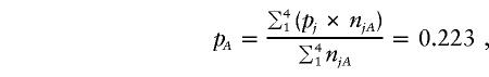
To answer this question, we first need to define “overall” prevalence. Most simply, it may be viewed as being the marginal mean of the true stratum-specific prevalences weighted by the number of individuals in each stratum:
 |
 |
The estimates we obtain using the Li-Mantel estimator and the Gibbs sampling model are both based on analyses conducted on the ascertained data set, and one might therefore anticipate that they should reflect the marginal distribution of stratum membership in the ascertained sample, not that in the original population. It would therefore seem reasonable to expect that the overall estimates of prevalence we obtain should pertain to the ascertained sample and not to the original population. The empirical evidence is clearly consistent with this surmise: the two estimates 0.238 and 0.245 are much closer to pA (0.223) than to pP (0.132). Furthermore, over a wide variety of simulated data sets, we have found this example to be typical and have found no case in which the empirical evidence is inconsistent with the conjecture.
This having been said, the analysis is poorly specified: no account has been taken of the real heterogeneity of risk arising from the effect of the unobserved strata. It could therefore be argued that, in this situation, the basic concept of “overall” prevalence is flawed. In essence, we are taking the weighted mean of a series of prevalence estimates that are, in actuality, different from one another. Although, at one level, this is true, the reality is that when we deal with complex diseases it is likely that many of the parameters that we estimate in our day-to-day work are marginal expectations of stratum-specific parameters of this type—it is just that, most of the time, we do not know enough about the etiological determinants to resolve the strata. Given that this is so, it is reassuring that, despite the extreme heterogeneity of the stratum-specific prevalences in the ideal example we have constructed and the marked difference between the marginal distribution of strata in the ascertained sample and the original population from which it was drawn, both the classical and Gibbs sampling estimators appear to provide good approximations to the true “overall” prevalence in the ascertained subpopulation. In the complete absence of knowledge of the determinants that generate a risk-stratification structure, one can ask for no more than a statistic that provides an acceptable summary across the strata.
Example 2: Predicting the Parameter Estimates in a Variance-Component Model Fitted to Simulated Ascertained Data
For our second example, we turn to the practical problem that first drew our attention to the issues we discuss in this article. That is, we address the apparent bias of parameter estimates relative to simulated population values that we found when we attempted to fit ascertainment-adjusted genetic variance-component models to simulated ascertained data. We will assume the following model of disease (D) generation:
 |
Here, i and j index the jth member of the ith sibship, α is the grand mean, z is a vector of observed covariates (centered about their means), and β is a corresponding vector of unknown fixed regression coefficients. Ci is a Normally distributed random effect shared by all members of the ith sibship, and Dij is a binary disease indicator (0 = unaffected; l = affected). In the conventional terminology of generalized linear models (McCullagh and Nelder 1989), ηij is the linear predictor, the error structure is Bernoulli, and the link function is logit. The inclusion of the Ci random effects in the linear predictor makes this a generalized linear mixed model (GLMM) (Breslow and Clayton 1993; Burton et al. 1999).
In a typical simulation, we sample 1,000 sibships, each of size five. We generate two observed covariates. One is binary [zb∼Bernoulli(0.3)], but, prior to analysis, it is centered about its mean by subtracting 0.3. The other is continuous [zq∼N(0,0.04)]. We set α=-5, βb=-0.4, βq=0.3, and σ2C=4.5. Under this model, most (nearly 90%) sibships that are generated have no affected members, but we ascertain only sibships with at least one affected member. We simulate complete ascertainment by sampling all such sibships.
The ascertainment mechanism will preferentially select sibships that, by chance, have a high value of the random effect Ci—that is, values of Ci that are sampled from the upper tail of the N(0,4.5) distribution. This has two effects. First, the mean of the true Ci values in the ascertained subpopulation is not 0 but, in this particular case, 2.76. Second, the variance of the true Ci values in the sample is not 4.5 but 2.42. On the other hand, perhaps counterintuitively, the empirical distribution of the sampled Ci values remains approximately Normal. The mean of the true ηij values in the ascertained sample is −2.23.
It is important to emphasize that the true values of the sampled Ci random effects and the ηij linear predictors to which we refer are the quantities that are generated by the simulation procedure, not the corresponding quantities that are estimated during the process of model fitting. Like the true stratum-specific prevalences in example 1, the true individual Ci and ηij values are unaffected by the process of ascertainment, but, for the reasons we specify, their marginal distributions are very different in the ascertained sample and in the original population.
We focus attention on estimates of the grand mean (α) and the variance (σ2C) of the Ci random effects. If our adjustment for ascertainment returned general population values, then, given that the fixed covariates are centralized about their means, one would expect an ascertainment-adjusted analysis to return the simulated values: α=-5 and σ2C=4.5 (or, to be more precise, −4.98 and 4.38, which, in this particular case, are the empirical mean of the true ηij values and the empirical variance of the true Ci values in the original simulated population prior to ascertainment). On the other hand, if an ascertainmnet-adjusted analysis returned estimates of true parameter values in the ascertained subpopulation, one would expect the estimated grand mean ( ) to reflect the true mean of the ηij in the ascertained sample (−2.23) and
  to reflect the true variance of the Ci values in the sample (2.42). In the complete absence of any adjustment for ascertainment, one would expect a marked overestimate of α, which would have the effect of making familial “clusters” of affected individuals seem unsurprising and would therefore lead to a marked underestimate of σ2C.
Analysis was based on the Gibbs sampling methods for clustered binary responses, which we have described elsewhere (Burton et al. 1999). An adjustment for ascertainment was introduced by dividing the unconditional Bernoulli likelihood by the probability of ascertainment on the basis of the parameters of the model. This adjustment was implemented in WinBUGS using the “ones trick” (Spiegelhalter et al. 2000), which introduces a Metropolis-Hastings step equivalent to that used in the simple model detailed in Appendix B. This can be viewed as being an Markov chain Monte Carlo analogue of the likelihood-based adjustment for complete ascertainment described by Elston and Sobel (1979).
In the event, without adjustment for ascertainment, the estimated values were  and
and  , which are both biased in the expected directions. Having adjusted for ascertainment, the estimated values were
  (SE 0.12) and
  (SE 0.36). These latter estimates reinforce the message that our ascertainment adjustment returns estimates of true parameter values in the ascertained subpopulation (α=-2.23 and σ2C=2.42), not in the general population (α=-4.98 and σ2C=4.38). As before, despite carrying out a wide range of different simulations, we found no case in which these conclusions were contradicted.
It has already been shown that GLMMs of this class generate consistent parameter estimates for correlated binary data (Burton et al. 1999). Nevertheless, to check that our basic model generates sensible estimates in this particular setting, we fitted a GLMM (without ascertainment adjustment) to the full original population (as it was prior to ascertainment). This returned the estimates  (SE 0.092) and
  (SE 0.284).
Discussion
In addressing the question of whether ascertainment-adjusted parameters estimates reflect true values in the sample or in the population from which the sample was ascertained, we have shown that two different situations exist. If one is estimating a parameter that is itself unaffected by the ascertainment, the true values in the sample and in the original population will be the same, and inferences apply to either population. On the other hand, if the true value of a parameter of interest differs between the general population and the ascertained subpopulation, an analysis based on the ascertained subpopulation will return an estimate of the true parameter value in the sample, not in the original population. The situation in which such an eventuality is most likely to occur is when the parameter of interest is the marginal expectation of a parameter across a number of strata. If this is so, and if the ascertainment influences the marginal distribution of strata (as it almost always will do if stratum membership is related to the risk of affectation), then parameter values will differ between the ascertained subpopulation and the original population. In such a situation, a standard ascertainment-adjusted analysis will estimate parameter values in the ascertained sample, not in the original population.
This has important implications for studies of complex diseases. Given that many of the etiological determinants of most complex diseases are unknown, it is safest to assume that, after taking account of determinants that are known, there could remain potentially strong risk stratification within the general population, based on unknown determinants. If an ascertained subpopulation is now drawn, high-risk strata will be overrepresented in the sample, and an ascertainment-adjusted estimate of prevalence based on that sample will reflect the higher true prevalence in the ascertained subpopulation and not that in the general population. Similarly, if scientific interest focuses on the relative risk associated with an observed determinant—for example, the ratio of risks associated with two different alleles at a genotyped locus—and the true relative risk associated with this determinant varies across different strata defined by other unknown determinants (reflecting, for example, epistatic or gene-environment interaction), the same phenomenon will occur. The ascertainment-adjusted relative risk will reflect the true relative risk in the ascertained subpopulation and not that in the original population.
In consequence, even when what are thought to be appropriate ascertainment adjustments have been applied, it is possible that two samples ascertained in different ways from the same underlying population will generate different estimates for what might appear to be the same parameter. Furthermore, despite adjustment for ascertainment, a parameter estimate based on a randomly sampled population need not be the same as its equivalent from an ascertained population. This has obvious implications not only for the interpretation of individual studies but also for the pooling of estimates within a meta-analysis. Another way of expressing the implications of this article is that it is simply not possible, using a conventional ascertainment adjustment, to consistently estimate a general population parameter in the presence of substantial latent etiological heterogeneity.
That there can be misunderstanding about these issues is in part a reflection of the fact that many of the traditional methods of adjustment for ascertainment (Fisher 1934; Li and Mantel 1968; Elston and Sobel 1979) were developed at a time when most of the conditions of interest could reasonably be assumed to be caused by one principal determinant (genetic or environmental). Under such circumstances, once one had modeled the effect of the determinant of interest and had incorporated an appropriate adjustment for ascertainment, any residual stratification consequent on unobserved determinants (of risk or of relative risk) would have been weak or absent. Many of the classical papers introducing ascertainment adjustments (Fisher 1934; Li and Mantel 1968) address the calculation of segregation ratios, so as to determine whether observed data are consistent with a recessive mode of inheritance attributable to a single gene. Under such circumstances, the concept that there could be latent stratification in the population such that, in some strata, the prevalence of affection (and therefore the “true” segregation ratio) is really 0.1, whereas in others it is 0.5, would have made little or no sense. However, given the current focus on complex diseases, in which unobserved stratification is likely to be the rule rather than the exception, it seems safer to assume that inferences pertain to parameter values in the ascertained subpopulation and not in the general population from which the ascertained subpopulation was drawn.
To finish, we reexamine the historical perspective. Although we would argue that the specific issue we address has received inadequate attention in the statistical genetics literature, we acknowledge that Greenberg and Hodge (1985) highlight the distinction between estimating population- and sample-based parameters. They describe an ascertainment-adjusted segregation analysis model for a recessive disease with a gene frequency q and a frequency R of sporadic cases in the general population. They focus on the estimation of α: the data set (sample) proportion of families in which the disease is genetic. They find marked biases in the estimates of q and R and conclude that “[t]he fact that α can be more accurately estimated than q or R may be due to the fact that it is a data set–based parameter, not a population-based one.” However, no explanation is provided as to why that might, in general, be so. Our article provides an explanation. Furthermore, we note that a different, although related, issue was raised by Fisher in his seminal paper in 1934. In trying to determine what estimate of p′ (“the probability of an affected individual being bought into the record”) to insert into his formula for the variance of the segregation ratio, in a situation in which there was marked heterogeneity in the probability of ascertainment in different subsets of the ascertainable population, he noted that “the estimate required is the true probability of ascertainment averaged, if heterogeneous, on the numbers of defectives ascertained, and not on the numbers available for ascertainment” (Fisher 1934).
Finally, we have very recently become aware of important preliminary work (Pfeiffer et al. 2000) that is relevant to what we have written. Example 2 differs from example 1, in that the latent heterogeneity is modeled in full by a parameter (σ2C) that is included in the model. Consequently, although our Gibbs sampling–based model returns sample-based parameter estimates, an alternative maximum likelihood–based model could be envisaged that would return approximate population-based parameter estimates (Pfeiffer et al. 2000). However, when the latent heterogeneity is not modeled at all, as in example 1, or is modeled incompletely, as will generally be the case in studies of complex diseases, estimates will always and in principle be sample based and not population based.
Acknowledgments
The methodological research in genetic epidemiology underpinning this work was funded by the National Health and Medical Research Council of Australia (NH&MRC) under program grant 00/3209, the National Center for Human Genome Research under Public Health Service grant HG01577, the National Institute of General Medical Sciences under Public Health Service grant GM28356, and the National Center for Research Resources under resource grant RR0365. L.J.P. is a NH&MRC Postdoctoral Research Fellow in Genetic Epidemiology, a Winston Churchill Memorial Trust Churchill Fellow, and an Australian-American Educational Foundation Fulbright Fellow. We are grateful to two anonymous reviewers whose constructive comments were very helpful in preparing the paper for publication.
Appendix A: Adjusting for Complete Ascertainment: the Li and Mantel (1968) Estimator
We wish to estimate the prevalence of a disease D, given information on a population of sibships (each of size three) that fall into four distinct risk strata, 1–4. Stratum membership is the only determinant of risk for the disease. We denote the true prevalence of D in the four strata as p1...p4. We require stratum-specific prevalence estimates ( ), but our data are restricted to sibships with at least one affected member. Ascertainment is complete—that is, all affected individuals are ascertained, and the sample consists of all sibships with at least one affected member. Denote by njk the number of sibships that are in risk stratum j and have k affected members. For k⩾1, the number of such sibships is the same in the ascertained sample as in the original population.
Denote by njA the total number of sibships in stratum j in the ascertained sample (njA=nj1+nj2+nj3) and by njP the number in the original population (njP=nj0+nj1+nj2+nj3). Denote by mjA and mjP the equivalent number of individuals: mjA=3×njA and mjP=3×njP. Finally, denote by ajA (or, equivalently, ajP) the number of affected individuals in the sample (or in the original population): ajA=ajP=(1×nj1)+(2×nj2)+(3×nj3).
Given pj, the probability that any one sibship in stratum j would have been ascertained is 1-(1-pj)3. In the absence of knowledge of nj0, but given pj, the total number of sibships in stratum j in the original general population can therefore be inferred to have been
The expected number of affected individuals in stratum j is
The expected number of sibships in stratum j with exactly one affected member is
The expected number of children (affected or not) in the ascertained sample can be obtained by rearranging equation (1) and multiplying by 3:
Now, let us consider the following expression:
Substituting in from equations (2), (3), and (4), this may be expanded to
But pj is the quantity we wish to estimate, and, if expectations are replaced by observed values, expression (5) can be used to derive a simple estimator for pj:  . We refer to this as the “Li-Mantel estimator.” If one denotes
  , Li and Mantel (1968) show that an asymptotic variance estimate for
  is given by
  .
.
Appendix B: Adjusting for Complete Ascertainment
Gibbs Sampling–Based WinBUGS Model
Random Number Generating Seeds for Five Separate Analyses:
stratum 1 analysis 73741
stratum 2 analysis 73742
stratum 3 analysis 73743
stratum 4 analysis 73744
all strata analysis 73745
Data for Five Separate Analyses:
stratum 1 analysis list(N=c(763,49,1));
stratum 2 analysis list(N=c(446,61,3));
stratum 3 analysis list(N=c(333,105,11));
stratum 4 analysis list(N=c(312,288,88));
all strata analysis list(N=c(1854,503,103))
Initial Values for P (Analysis Based on Three Independent Chains):
list(p=0.01);
list(p=0.2);
list(p=0.5);
Model:
model
{
#Calculate Binomial likelihoods associated with 1, 2, and 3 affected siblings in a sibship
like.sibship[1] <- 3*pow(p, 1)*pow((1-p),2);
like.sibship[2] <- 3*pow(p,2)*pow((1-p),l);
like.sibship[3] <- 1*pow(p,3);
#Calculate probability of ascertainment as a function of modeled prevalence parameter (p)
prob.asc<-(1 -(1-p)*(1-p)*(1-p));
#Model fitting loop
for(i in 1:3)
{
#Calculate conditional likelihoods by dividing likelihoods by probability of ascertainment
cond.like.sibship[i]<-like.sibship[i]/prob.asc;
#Combine conditional likelihood for sibships with i affected children across all sibships of that class
cond.like.total[i]<-pow(cond.like.sibship[i],N[i]);
#Fit model using a Metropolis Hastings step to deal with conditional likelihood (the “ones trick”)
ones[i]<-1;
ones[i]-dbern(cond.like.total[i]);
}
#Specify flat beta prior for p (uniform on the real line between 0 and 1)
p-dbeta(1,1);
}
Model Fitting
All of the WinBUGS analyses referred to in this article are based on three independent estimation chains run in parallel. The three chains are initialized using different starting values. Chains are run for 10,000 iterations following a discarded burn-in of 500 iterations. In every case, the chains exhibit good convergence and mixing. Vague priors are used throughout (Burton et al. 1999).
References
- Breslow NE, Clayton DG (1993) Approximate inference in generalized linear mixed models. J Am Stat Assoc 88:9–25 [Google Scholar]
- Burton PR (1994) Helping doctors to draw appropriate inferences from the analysis of medical studies. Stat Med 13:1699–1714 [DOI] [PubMed] [Google Scholar]
- Burton PR, Tiller K, Gurrin LC, Musk AW, Cookson WOCM, Palmer LJ (1999) Genetic variance components analysis for binary phenotypes using generalized linear mixed models (GLMMs) and Gibbs sampling. Genet Epidemiol 17:118–140 [DOI] [PubMed] [Google Scholar]
- Cannings C, Thompson EA (1977) Ascertainment in the sequential sampling of pedigrees. Clin Genet 12:208–212 [DOI] [PubMed] [Google Scholar]
- Elston RC (1995) ‘Twixt cup and lip: how intractable is the ascertainment problem? Am J Hum Genet 56:15–17 [PMC free article] [PubMed] [Google Scholar]
- Elston RC, Sobel E (1979) Sampling considerations in the gathering and analysis of pedigree data. Am J Hum Genet 31:62–69 [PMC free article] [PubMed] [Google Scholar]
- Ewens WJ, Shute NCE (1986) A resolution of the ascertainment sampling problem. 1. Theory. Theor Popul Biol 30:388–412 [DOI] [PubMed] [Google Scholar]
- Fisher RA (1934) The effect of methods of ascertainment upon the estimation of frequencies. Ann Eugenics 6:13–25 [Google Scholar]
- Greenberg DA, Hodge SE (1985) The heterogeneity problem. 1: Separating genetic from environmental forms of the same disease. Am J Med Genet 21:357–371 [DOI] [PubMed] [Google Scholar]
- Hodge SE (1988) Conditioning on subsets of the data: applications to ascertainment and other genetic problems. Am J Hum Genet 43:364–373 [PMC free article] [PubMed] [Google Scholar]
- Lalouel JM, Morton NE (1981) Complex segregation analysis with pointers. Hum Hered 31:312–321 [DOI] [PubMed] [Google Scholar]
- Li CC, Mantel N (1968) A simple method of estimating the segregation ratio under complete ascertainment. Am J Hum Genet 20:61–81 [PMC free article] [PubMed] [Google Scholar]
- Lindley DV (1965). Introduction to probability and statistics from a Bayesian viewpoint. Part 2. Inference. Cambridge University Press, Cambridge [Google Scholar]
- McCullagh P, Nelder JA (1989) Generalized Linear Models. Chapman and Hall, Oxford [Google Scholar]
- Pfeiffer R, Gail MH, Pee D (2000) Inference for environmental effects based on family data taking into account ascertainment and random genetic effects [abstract]. International Society for Clinical Biostatistics, Trento, Italy, September 2000 [Google Scholar]
- Spiegelhalter D, Thomas A, Best N (2000) WinBUGS version 1.3 user manual. MRC Biostatistics Unit, Cambridge [Google Scholar]
- Vieland VJ, Hodge SE (1995) Inherent intractability of the ascertainment problem for pedigree data: a general likelihood framework. Am J Hum Genet 56:33–43 [PMC free article] [PubMed] [Google Scholar]