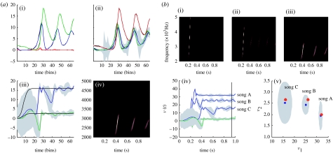
Figure 6.
(a) Schematic of perceptual categorization ((i) prediction and error, (ii) hidden states, (iii) causes and (iv) percept). This follows the same format as in figure 3. However, here, there are no hidden states at the second level and the causes were subject to stationary and uninformative priors. This song was generated by a first-level attractor with fixed control parameters of and , respectively. It can be seen that, on inversion of this model, these two control variables, corresponding to causes or states at the second level, are recovered with relatively high conditional precision. However, it takes approximately 50 iterations (approx. 600 ms) before they stabilize. In other words, the sensory sequence has been mapped correctly to a point in perceptual space after the occurrence of the second chirp. This song corresponds to song C (b(iii)). (b) The results of inversion for three songs ((i) song A, (ii) song B and (iii) song C) each produced with three distinct pairs of values for the second-level causes (the Rayleigh and Prandtl variables of the first-level attractor). (i–iii) The three songs shown in sonogram format correspond to a series of relatively high-frequency chirps that fall progressively in both frequency and number as the Rayleigh number is decreased. (iv) These are the second-level causes shown as a function of peristimulus time for the three songs. It can be seen that the causes are identified after approximately 600 ms with high conditional precision. (v) The conditional density on the causes shortly before the end of peristimulus time (vertical line in (iv)). The blue dots correspond to conditional means or expectations and the grey areas correspond to the conditional confidence regions. Note that these encompass the true values (red dots) used to generate the songs. These results indicate that there has been a successful categorization, in the sense that there is no ambiguity (from the point of view of the synthetic bird) about which song was heard.

