

Abstract
A general-purpose deformable registration algorithm referred to as “DRAMMS” is presented in this paper. DRAMMS bridges the gap between the traditional voxel-wise methods and landmark/feature-based methods with primarily two contributions. First, DRAMMS renders each voxel relatively distinctively identifiable by a rich set of attributes, therefore largely reducing matching ambiguities. In particular, a set of multi-scale and multi-orientation Gabor attributes are extracted and the optimal components are selected, so that they form a highly distinctive morphological signature reflecting the anatomical and geometric context around each voxel. Moreover, the way in which the optimal Gabor attributes are constructed is independent from the underlying image modalities or contents, which renders DRAMMS generally applicable to diverse registration tasks. A second contribution of DRAMMS is that it modulates the registration by assigning higher weights to those voxels having higher ability to establish unique (hence reliable) correspondences across images, therefore reducing the negative impact of those regions that are less capable of finding correspondences. A continuously-valued weighting function named “mutual-saliency” is developed to reflect the matching reliability between a pair of voxels implied by the tentative transformation. As a result, voxels do not contribute equally as in most voxel-wise methods, nor in isolation as in landmark/feature-based methods. Instead, they contribute according to the continuously-valued mutual-saliency map, which dynamically evolves during the registration process. Experiments in simulated images, inter-subject images, single-/multi-modality images, from brain, heart, and prostate have demonstrated the general applicability and the accuracy of DRAMMS.
Keywords: image registration, deformable registration, non-rigid registration, attribute matching, Gabor filter bank, Gabor attributes, feature selection, matching reliability, reliability detection, mutual saliency, missing data, loss of correspondence
1. Introduction
Image registration is the process of finding the optimal transformation that aligns different imaging data into spatial correspondence [Zitova and Flusser, 2003; Crum et al., 2004]. It is the building block for a variety of medical image analysis tasks, such as motion correction (e.g. [Zuo et al., 1996; Bai and Brady, 2009]), multi-modality information fusion (e.g., [Meyer et al., 1997; Verma et al., 2008]), atlas-based image segmentation (e.g., [Prastawa et al., 2005; Lawes et al., 2008; Gee et al., 1993]), population studies (e.g., [Geng et al., 2009; Sotiras et al., 2009; Ou et al., 2009b; Zollei et al., 2005]), longitudinal studies (e.g., [Csapo et al., 2007; Shen and Davatzikos, 2004; Xue et al., 2006]), computational anatomy (e.g., [Joshi et al., 2004; Ashburner, 2007; Leow et al., 2007; Thompson and Apostolova, 2007]) and image-guided surgery (e.g., [Muratore et al., 2003; Gering et al., 2001; Hata et al., 1998]). During the past two decades, a large number of deformable (non-rigid) image registration methods have been developed, and several thorough reviews can be found in [Maintz and Viergever, 1998; Lester and Arridge, 1999; Hill et al., 2001; Zitova and Flusser, 2003; Pluim et al., 2003; Crum et al., 2004; Holden, 2008].
These existing deformable registration methods can be generally classified into two main categories: landmark/feature-based methods and voxel-wise methods. Examples of the former category include [Thompson and Toga, 1996; Davatzikos et al., 1996; Rohr et al., 2001; Shen and Davatzikos, 2003; Joshi and Miller, 2000; Chui and Rangarajan, 2003; Zhan et al., 2007; Ou et al., 2009a; Gee et al., 1994], among others. Examples of the latter category include [Glocker et al., 2008; Vercauteren et al., 2007, 2009; Ou and Davatzikos, 2009; D'Agostino et al., 2003; Kybic and Unser, 2003; Christensen et al., 1994; Collins et al., 1994; Thirion, 1998; Rueckert et al., 1999; Maes et al., 1997; Wells et al., 1996; Friston et al., 1995], among others. Specifically, landmark/feature-based methods, the former category, often explicitly detect and establish correspondences on those anatomically and/or geometrically salient regions (e.g., surfaces, corners, boundary points, line intersections), and then spread the correspondences throughout the entire image space. This category of methods is fairly intuitive and computationally efficient, since only a small proportion of the imaging data detected as landmarks/features is used. However, they usually suffer from inevitable errors in the landmark/feature detection and matching processes, and suffer from the often non-uniform distribution of landmarks within the image space, which causes non-uniform distribution of registration accuracy. Another drawback is that, the choice of landmark/feature detection tools is usually heavily dependent on the specific contents of images being registered. For instance, the landmark/feature detection tool that is used to recognize the surface of corpus callosum for brain image registration tasks is usually quite different from the landmark/feature detection tool that is used to recognize nipples for breast image registration tasks. Because of all these reasons in landmark/feature-based methods, recent literature on general-purpose registration has mostly focused on voxel-wise methods, i.e., the second main category of registration methods, which usually equally utilize all imaging data and find the optimal transformation by maximizing an overall similarity defined on certain voxel-wise attributes (e.g., intensities, intensity distributions).
The general-purpose registration method proposed in this paper belongs essentially to voxel-wise methods. It is developed to overcome the following two limitations in traditional voxel-wise methods.
The first major limitation in traditional voxel-wise methods is that, they characterize voxels by attributes that are not necessarily optimal. Since the matching between a pair of voxels is based upon the matching between the attributes characterizing them, suboptimal attributes will unavoidably lead to matching ambiguities [Shen and Davatzikos, 2003; Xue et al., 2004; Wu et al., 2006; Liao and Chung, 2009]. Indeed, most voxel-wise methods characterize voxels only by image intensity; however, intensity attribute alone leads to large matching ambiguities – for instance, hundreds of thousands of gray matter voxels in a brain image would have similar intensities; but they all correspond to different anatomical regions. To reduce matching ambiguities, other methods (e.g., [Shen and Davatzikos, 2003]) attempted to characterize voxels by a richer set of attributes, such as surface curvatures and tissue membership. These attributes, although capable of reducing matching ambiguities, are often task- and parameter- specific, hence not generally applicable for diverse registration tasks. In this paper, we argue and demonstrate that, an ideal set of attributes should satisfy two conditions: 1) discriminative, i.e., attributes of two voxels will be similar if and only if they are anatomically corresponding to each other, therefore leaving minimum ambiguity in matching; 2) generally applicable, i.e., a good set of image attributes should be able to be extracted from almost all medical images, while still satisfying the first condition, regardless of the image modalities or contents. Finding a set of attributes that satisfy these two criteria and developing a method to select the best components thus become the first major contribution in this paper.
The second major limitation of traditional voxel-wise methods is that, they often utilize all imaging data equally, which usually undermines the performance of the optimization process. Actually, different anatomical regions/voxels usually have different abilities to establish unique correspondence [Anandan, 1989; McEachen and Duncan, 1997; Wu et al., 2007]. An obvious example is when there is missing data, or loss of correspondence. For instance, in Fig. 1, the lesion regions in the diseased brain image (subject) could hardly find correspondences in the normal brain image (template). In a more general setting, even if there is no missing data or loss of correspondence, certain parts of the anatomy are still more easily identifiable than others. In Fig. 2, for instance, three voxels (depicted by red, blue and orange crosses) are examined. A similarity map is generated by calculating attribute-based similarity between one of these three voxels in the subject image and all voxels in the template image. The similarity maps (Fig. 2(c)(d)(e)) reveal a smaller number of matching candidates for the red point, more candidates for the blue point and much more candidates for the yellow point. This indicates their different abilities to establish unique correspondences, or conversely, different degrees of matching ambiguities. Naturally, these three points should be treated with different “confidences” during registration. Unfortunately, most voxel-wise methods, such as the mutual-information based methods, treat all voxels equally, ignoring such differences. Other approaches attempted to address this issue, by driving the registration adaptively/hierarchically using certain anatomically salient regions. However, in their approaches only a small proportion of voxels are finally utilized, and the potential contributions from other non-utilized voxels are ignored. Moreover, the determination of which voxels to be utilized and which not is largely heuristic or dependent on the a priori knowledge. In this paper, we propose and demonstrate that, an ideal optimization process should utilize all imaging voxels, but with different weights, based on their abilities to establish unique correspondences across images. This is important for increasing the matching reliability in general, and for minimizing the negative impact of the loss of correspondence (or missing data) when they exist (like in Fig. 1).
Figure 1.

Need for weighting voxels differently when there is partial loss of correspondence. The lesion (white region) in the subject image is less capable of establishing unique correspondences across images and hence should be assigned with lower weights to reduce its negative impact to registration process.
Figure 2.

Need for weighting voxels differently in a typical image registration scenario. Similarity maps (c-e) are generated between one specific voxel (depicted by red, blue and orange crosses) in the subject image (a) and all voxels in the template image (b). The red point has higher ability to establish unique correspondences, hence should be assigned with higher weight during registration, followed by blue point and orange point in descending order. This figure is better viewed in color version.
In this paper, we present DRAMMS – Deformable Registration via Attribute Matching and Mutual-Saliency Weighting – to overcome these two aforementioned limitations. To overcome the first limitation, DRAMMS extracts a rich set of multi-scale and multi-orientation Gabor attributes at each voxel and automatically selects the optimal attributes. The optimal Gabor attributes render it relatively robust in attribute-based image matching, and are also constructed in a way that is readily applicable to various image contents and image modalities. To overcome the second limitation, DRAMMS continuously weights voxels during the optimization process, based on a function referred to as “mutual-saliency”. Mutual-saliency measure quantifies the matching uniqueness (hence reliability, used thereafter interchangeably) between a pair of voxels implied by the transformation. In contrast to equally treating voxels or isolating voxels that have more distinctive attributes, this mutual-saliency based continuous weighting mechanism utilizes all imaging data with appropriate and dynamically-evolving weights and leads to a more effective optimization process.
This paper is an augmented version of a previously published conference version [Ou and Davatzikos, 2009]. The extensions include more detailed method descriptions, more validations and more thorough discussions. Also, the gradient-descent-based optimization strategy in the conference version has now been replaced by the state-of-the-art discrete optimization strategy [Komodakis et al., 2008], leading to higher speed while maintaining registration accuracy. We also refer to HAMMER registration method [Shen and Davatzikos, 2003], which is closely related to our work, and the difference between DRAMMS and HAMMER is discussed in Section 5.5.
In the remainder of this paper, DRAMMS is elaborated in Section 2, with implementation details in Section 3 and experimental results in Section 4. The whole paper is discussed and concluded in Section 5.
2. Methods
2.1. Problem Formulation
Given two intensity images I1 : Ω1 ↦ ℝ and I2 : Ω2 ↦ ℝ in 3D image domains Ωi(i = 1, 2) ⊂ ℝ3, DRAMMS seeks a transformation T that maps every voxel u ∈ Ω1 to its counterpart T(u) ∈ Ω2, by minimizing an overall cost function E(T),
| (1) |
where (i = 1, 2) is the optimal attribute vector that reflects the geometric and anatomical contexts around voxel u, and d is its dimension. By minimizing , we seek a transformation T that minimizes the dissimilarity between a pair of voxels u ∈ Ω1 and T(u) ∈ Ω2. The extraction of attributes and selection of optimal attribute vector (i = 1, 2) will be detailed in Sections 2.2.1 and 2.2.2.
ms (u, T(u)) is a continuously-valued weight that is calculated from the mutual-saliency between two voxels u ∈ Ω1 and T(u) ∈ Ω2 – higher uniqueness (reliability) of their matching in the neighborhood indicates higher mutual-saliency, and hence higher weight in the optimization process. The definition of mutual-saliency will be discussed in Section 2.3.
R(T) is a smoothness/regularization term usually corresponding to the Laplacian operator, or the bending energy [Bookstein, 1989], of the deformation field T, whereas λ is a balancing parameter that controls the extent of smoothness. Such a choice of regularization is widely adopted in numerous registration methods.
In accordance to the overall cost function in Eqn. 1, the framework of DRAMMS is also sketched in Fig. 3. The two major components – optimal attribute matching (AM) and mutual-saliency (MS) weighting – will be detailed in the subsequent sections 2.2 and 2.3.
Figure 3.

DRAMMS framework. “AM” stands for attribute matching and “MS” stands for mutual-saliency weighting. They are two major components in DRAMMS and will be described in detail in the subsequent sections 2.2 and 2.3.
2.2. Attribute Matching (AM)
This section will address the first major component of DRAMMS, namely, attribute matching (AM). The aim is to extract and select the optimal attributes that can reflect the geometric and anatomic contexts of each voxel, and at the same time, to keep the attribute extraction and selection readily applicable to diverse registration tasks. This component consists of two modules: attribute extraction (described in section 2.2.1) and attribute selection (described in section 2.2.2).
2.2.1. Attribute Extraction
The idea of characterizing each image voxel with a rich set of attributes has been previously explored in the community. In their pioneer work, [Shen and Davatzikos, 2003] incorporated geometric-moment-invariant (GMI) attributes, tissue membership attributes and boundary/edge attributes into a high-dimensional attribute vector to better characterize a voxel in human brain images. Since then, a number of geometric and texture attributes have been explored, including, but by no means limited to, intensity attributes (e.g., [Ellingsen and Prince, 2009; Foroughi and Abolmaesumi, 2005]), boundary/edge attributes (e.g., [Shen and Davatzikos, 2003; Zacharaki et al., 2008; Sundar et al., 2009; Ellingsen and Prince, 2009]), tissue membership attributes (requiring task-specific segmentation) (e.g., [Shen and Davatzikos, 2003; Xing et al., 2008; Zacharaki et al., 2008; Ellingsen and Prince, 2009]), wavelet-based attributes (e.g., [Xue et al., 2004]), local frequency attributes (e.g., Liu et al. [2002]; Jian et al. [2005]), local intensity histogram attributes (e.g., [Shen, 2007; Yang et al., 2008]), geodesic intensity histogram attributes (e.g., [Ling and Jacobs, 2005; Li et al., 2009]), tensor orientation attributes (specifically for diffusion tensor imaging registration) (e.g., [Verma and Davatzikos, 2004; Munoz-Moreno09 et al., 2009; Yap et al., 2009]), and curvature attributes (specifically for surface matching) (e.g., [Shen et al., 2001; Liu et al., 2004; Zhan et al., 2007; Ou et al., 2009a]). These studies have all demonstrated improved registration accuracies as a result of more distinctive characterizations of voxels. However, as most of these attributes are pre-conditioned on segmentation, tissue labeling, or edge detection, and are tailored to specific image content or modality, there is still need to systematically find a common set of attributes that are generally applicable for various image contents. And also, there is need to automatically, other than heuristically, select the optimal attribute components. DRAMMS aims in this direction. In particular, DRAMMS extracts a set of multi-scale and multi-orientation Gabor attributes at each voxel by convolving the images with a set of Gabor filter banks.
The use of Gabor attributes in DRAMMS is mainly motivated by the following three properties of Gabor filter banks:
General applicability and successful application in numerous tasks. Almost all anatomical images have texture information, at some scale and orientation, reflecting the underlying geometric and anatomical characteristics. This texture information can be effectively captured by Gabor attributes, as demonstrated in a variety of studies, including texture segmentation (e.g., [Jain and Farrokhnia, 1991]), image retrieval (e.g., [Manjunath and Ma, 1996]), cancer detection (e.g., [Zhang and Liu, 2004]) and tissue differentiation (e.g., [Zhan and Shen, 2006; Xue et al., 2009]). Recently, Gabor attributes have also been successfully used in [Liu et al., 2002; Verma and Davatzikos, 2004; Elbakary and Sundareshan, 2005] to register images of different contents/organs. This promises the use of Gabor attributes for a variety of image registration tasks. The previous methods have also pointed out some drawbacks related to the use of Gabor attributes, such as the high computational cost and the need for an appropriate choice of attribute components due to the conveyed redundant information. DRAMMS addresses both drawbacks by developing a module for selecting the optimal Gabor components, which will be detailed in Section 2.2.2.
Suitability for single- and multi-modality registration tasks. This is mainly because of the multi-scale property in Gabor filter banks. Specifically, those high-frequency Gabor filters often serve as edge detectors, detected edge information is, to some extent, independent of the underlying intensity distributions, and is therefore suitable for multi-modality registration tasks. This holds even when intensity distributions in the two images no longer follow consistent relationship, in which case mutual-information [Wells et al., 1996; Maes et al., 1997] based methods are challenged [Liu et al., 2002]. On the other hand, the low-frequency Gabor filters often serve as local image smoothers, and the corresponding attributes are analogous to images at coarse resolutions, which will largely help prevent the cost function from being trapped at the local minima. As a demonstration Fig. 4 shows a typical set of high- and low-frequency Gabor attributes for two typical human brain images from different modalities. In this case, edge information extracted by high-frequency Gabor filters (first row in the figure) provides basis for the multi-modality registration.
Multi-scale and multi-orientation nature. As [Kadir and Brady, 2001] pointed out, scale and orientation are closely related to the distinctiveness of attributes. The multi-scale and multi-orientation attributes are more likely to render each voxel distinctively identifiable, therefore reducing ambiguities in attribute-based voxel matching. For instance, compared with traditional edge detectors (e.g., Canny, Sobel), the multi-orientation Gabor attributes will easily differentiate edges in horizontal and vertical directions (see Fig. 4).
Figure 4.

Multi-scale and multi-orientation Gabor attributes extracted from two typical human brain images. To save space, shown here are only representative attributes from the real part of three orientations (π/2, π/3 and π) in the x-y plane (a full set of Gabor attributes is mathematically described in Eqn. 6).
Direct computation of 3D Gabor attributes is usually time consuming. To save computational cost, the approximation strategy in [Manjunath and Ma, 1996; Zhan and Shen, 2006] is adopted in this paper. Specifically, the 3D Gabor attributes at each voxel are approximated by convolving the 3D image with two groups of 2D Gabor filter banks in two orthogonal planes (x-y and y-z planes). Mathematically, the two 2D Gabor filter banks in two orthogonal planes are
| (2) |
| (3) |
where a is the scale basis set to 2 for image re-sampling. m = 1, 2, …, M is the index for scales, with M being the total number of scales; as m varies, the scale factor am leads to different sizes of the neighborhood from which the multi-scale Gabor attributes are extracted. , , and are rotated coordinates, where n = 1, 2, …, N is the index for orientations, with N being the total number of orientations. As n varies, Gabor envelops rotate in x-y and y-z planes, leading to multi-orientation Gabor attributes.
g(x, y) and h(y, z) in the equations above are known as the “mother Gabor filters”, which are complex-valued functions in the spatial domain. They are each obtained by modulating a Gaussian envelope with a complex exponential. Intuitively, they are elliptically-shaped covers (Gaussian envelops) that specify the neighborhood of each voxel, from which the Gabor attributes will be extracted. Mathematically, the mother Gabor filters g(x, y) and h(y, z) are expressed as
| (4) |
| (5) |
where σx, σy and σz are the standard deviations of the Gaussian envelope in the spatial domain; fx and fy are modulating (shifting) factors in the frequency domain (often known as “central frequencies”) [Kamarainen, 2003].
As a result of attribute extraction, each voxel u = (x, y, z) will be characterized by a Gabor attribute vector Ãi(u) with dimension D = M × N × 4, as denoted in Eqn. 6. Here the factor 4 is because of two parts (real and imaginary) of Gabor responses from two orthogonal planes.
| (6) |
We call this attribute vector Ã(·) a “full” Gabor attribute vector, in contrast to the “optimal” attribute vector A⋆(·) to be selected in Section 2.2.2. The numbers of their dimensions are denoted as D and d, respectively, whereas D is determined by the number of scales and orientations (D = M × N × 4), and d is determined automatically during the subsequent attribute selection process.
Note that in Eqn. 6, we have taken magnitude (absolute value) of the Gabor response in the real and imaginary parts, therefore even contrast changes, the edge information extracted by high-frequency Gabor filters will remain stable, which is suitable for multi-modality registration.
Role of Full Gabor Attributes
Before selecting optimal attributes and using attribute vector for across-image matching, we need to make sure that the extracted full attribute vector Ãi(u) in Eqn. 6 is able to characterize voxels distinctively, at least within the image itself. By distinctive characterization, we mean that attributes of a point should be only similar (or identical) to attributes from the point itself, and should be different from attributes of any other voxels in the same image. In Fig. 5, two special points (labelled by red and blue crosses in sub-figure (a)) and two ordinary points (labelled by orange and purple crosses in sub-figure (a)) are examined in a typical brain MR image. Similarity maps (b,c,d,e) are calculated between the attributes of each of these examined voxels and attributes of all other voxels in the same image. From these similarity maps it can be observed that, both special voxels and ordinary voxels have been well localized with fairly small ambiguities by the full Gabor attributes Ãi(u).
Figure 5.
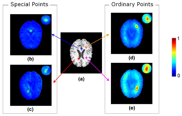
Role of full Gabor attributes in characterizing voxels relatively distinctively. Similarity maps (b-e) are created by calculating attribute-wise similarity between a single point (depicted by red, blue, orange or purple crosses in (a)) with all points in the same image. Compared to intensity attribute, the full Gabor attribute vector described in Eqn. 6 has led to far smaller number of voxels that are similar to the points being examined.
2.2.2. Attribute Selection
A disadvantage of Gabor attributes is the redundancy among attributes, which is largely caused by the non-orthogonality among Gabor filters at different scales and orientations. This redundancy not only increases computational cost, but more importantly, it may reduce the distinctiveness of attribute representation, causing ambiguities in the attribute matching [Manjunath and Ma, 1996; Kamarainen, 2003]. A learning-based method is therefore designed to select the optimal components.
The main idea of attribute selection is the following: if provided with some pairs of corresponding voxels from the two images, we can treat them as training samples and employ a machine learning method to select the optimal attribute components, such that their matching similarity and uniqueness are preserved or increased.
Two issues sit in the center of formulating this idea: 1) selection of training voxel pairs – in the context of general-purpose registration algorithm like ours, they should be selected right from the images being registered and the selection should be fully automatic without assumption of any a prior knowledge. Moreover, representative voxel pairs should be those that have high matching similarity and uniqueness; 2) selection of optimal attributes – here the criterion is to preserve or increase the matching similarity and uniqueness between these training voxel pairs.
Both issues rely on the quantifications of matching similarity and matching uniqueness between voxel pairs. Matching similarity sim(p, q) between a pair of voxels (p ∈ Ω1, q ∈ Ω2) can be defined based on their attribute vectors,
| (7) |
where smaller Euclidean distance between two attribute vectors indicate higher similarity. Note that the squared Euclidean distance between two attribute vectors is normalized by their dimensionality D, so as to make the similarity calculated from different number of attributes comparable. Matching reliability can be encoded by the mutual-saliency weight ms(·, ·), which will be elaborated in the subsequent section 2.3. With these quantifications, we can proceed to the two steps towards selecting optimal Gabor attribute components.
Step 1: Selecting Training Voxel Pairs
To encourage the training voxel pairs to represent all other voxels, they should be scattered in the image domain and far away from each other. Accordingly, DRAMMS regularly partitions the subject image I1 into a number of J regions and selects from each region a voxel pair that has highest matching similarity and matching uniqueness (measured by mutual-saliency), under the full Gabor attributes. Mathematically,
| (8) |
Note that the full Gabor attribute vector Ã(·) is used at this step, since no optimal components have been selected. The mutual-saliency measure ms(p, q) will be elaborated in a later Section 2.3; for now, the bottom line is that it reflects the matching uniqueness between p ∈ Ω1 and q ∈ Ω2.
Fig. 6 illustrates the selection of training voxel pairs. Here regular partition is used instead of more complicated organ/tissue segmentation, in order to keep DRAMMS as a general-purpose registration method without assumptions on segmentation. Note also that the template image I2 is not partitioned because at this stage, no transformation is performed and no corresponding regions should be assumed.
Figure 6.

Sketch of the selection of representative training voxel pairs, Ωi (i = 1, 2) are image spaces where two images Ii (i = 1, 2) reside. are J pairs of voxels that have been selected with highest matching similarity and highest matching uniqueness (measured by mutual saliency).
Step 2: Selecting Optimal Attributes
Once training voxel pairs have been determined, DRAMMS selects a subset of optimal attribute components A⋆() out of the full Gabor attribute vector Ã(), such that they maximize the overall similarity and matching uniqueness on these selected training voxel pairs. Mathematically,
| (9) |
Like in Eqn. 8, ms(·, ·) is the mutual-saliency that reflects the matching uniqueness and will be elaborated in the subsequent Section 2.3.
Actually, Eqn. 8 and Eqn. 9 share almost the same objective function [sim(·, ·) × ms(·, ·)]. Difference is that, in Eqn. 8, the full attribute vector Ã(·) is given and held unchanged, and the objective function is optimized over candidate voxel pairs to select best suitable training pairs; in Eqn. 9, on the other hand, the training voxel pairs are held unchanged and the objective function is optimized over candidate attributes to select a set of optimal attribute components.
To implement Eqn. 9, DRAMMS adopts an iterative backward elimination (BE) and forward inclusion (FI) strategy for attribute selection. Such a strategy is commonly used for attribute/variable selection in the machine learning community (e.g. [Guyon and Elisseeff, 2003; Fan et al., 2007]). The iterative process is specified as follows. Starting from a full set of D Gabor attributes Ã(·), each time we eliminate one Gabor component such that the objective function [ms(·, ·) × sim(·, ·)] increases by a larger amount than eliminating other components (this is known as backward elimination). We continue the elimination until there is no one to be eliminated (meaning that, eliminating any one attribute component will lead to decrease of the objective function). This ends one round of backward elimination. Staring from there, we start to include the previously-eliminated Gabor components once at a time, so that the cost function [ms(·, ·) × sim(·, ·)] increases by a largest amount than including other components (this is known as forward inclusion). We keep on this inclusion until there is no one to be included (meaning that, including any one attribute component will lead to decrease of the objective function). This ends one round of forward inclusion. Finally, we iterate between backward elimination and forward inclusion and monotonically increase the objective function, until there is no attribute component to be eliminated or included. Convergence is guaranteed as the number of attributes is bounded below and above. Upon convergence, the objective function [ms(·, ·) × sim(·, ·)] is maximized and the remaining attributes are the optimal set of attributes we will eventually use for attribute matching, denoted as A⋆(·). Fig. 7 shows a typical attribute selection process for two cardiac images being registered. In this case, the objective function keeps increasing during one round of BE process (where 39 attributes were eliminated from the full attribute set), one round of FI process (where 9 previously-eliminated attributes were included back to the remaining attribute set), and one more round of BE processes (where 4 attributes were eliminated from the attribute set), until it reaches the maximum, and then the optimal attribute set has been selected.
Figure 7.

A typical scenario for attribute selection. (a) The value of the objective function [ms(,) × sim(,)] with regard to the iteration index. (b) The number of attributes selected with regard to the iteration index. Starting from a full set of attributes, iterative backward elimination (BE) and forward inclusion (FI) processes are employed to select the optimal attributes. The objective function increases monotonically until no other attribute could be eliminated or included to increase it further. When the cost function stops increasing, the corresponding attributes are the ones selected as the optimal set.
Role of Optimal Gabor Attributes
Fig. 8 compares the intensity attribute, gray-level-cooccurance-matrix (GLCM) texture attributes [Haralick, 1979], full Gabor attributes, and the optimized Gabor attributes, in terms of matching ambiguities caused by different attributes. Similarity maps have been generated by these attributes between a special/ordinary point in the subject brain/cardiac image and all points in the template image. The optimal Gabor attributes lead to highly distinctive attribute characterizations, with less matching candidates both for a special point (depicted by the red cross) and for an ordinary point (depicted by blue cross). Since the similarity map for a given voxel now looks more like a “delta” function in the neighborhood of this voxel, the optimal Gabor attributes show great promise in reducing the risk of being trapped at local minimum.
Figure 8.

Role of attribute selection in reducing matching ambiguities, as illustrated on special voxels (red crosses) and ordinary voxels (blue crosses) in brain and cardiac images of different individuals. Similarity maps are generated between a voxel (red or blue) in the subject image and all voxels in the template image. “GLCM”, gray-level co-occurrence matrix [Haralick, 1979], is another commonly used texture attribute descriptor.
2.3. Using Mutual-Saliency Map to Modulate Registration
The above Section 2.2 has described extracting a full set of Gabor attributes (2.2.1) and selecting the optimal Gabor attributes (2.2.2) to characterize each voxel distinctively. That finishes the first component of DRAMMS, namely, attribute matching (AM). This section will elaborate the second component of DRAMMS, namely, mutual-saliency (MS) weighting, to better modulate the registration process.
As addressed in the introduction, an ideal optimization process should utilize all voxels but assign a continuously-valued weight to each voxel, based on the capability of this voxel to establish unique correspondences across images. Actually, the idea of reliability detection for better matching was probably first investigated in [Anandan, 1989; Duncan et al., 1991] and their follow-up studies [McEachen and Duncan, 1997; Shi et al., 2000]. They developed a “confidence” quantity for motion tracking on surface points, which measures whether the matching of two surface points are unique (reliable) in the neighborhood, based on the similarity defined on their curvatures. Other works explicitly segment the regions of interest in a joint segmentation and registration framework [Yezzi et al., 2001; Wyatt and Nobel, 2003; Chen et al., 2005; Pohl et al., 2006; Wang et al., 2006; Xue et al., 2008; Ou et al., 2009a]. Both approaches assign weights to certain feature voxels/regions depending on detection or segmentation, and are therefore not generally applicable to diverse tasks. For extension, we aim to develop a quantity that measures matching uniqueness (hence reliability) for every single voxel in the image and the quantification method should not be dependent on any prerequisite detection or segmentation.
Recent work [Huang et al., 2004; Bond and Brady, 2005; Yang et al., 2006; Wu et al., 2006; Mahapatra and Sun, 2008] assumed that more salient regions could establish more reliable (unique) correspondence and hence should be assigned with higher weights. As a result, improved registration accuracies have been reported. However, this intuitive assumption does not always hold, because regions that are salient in one image are not necessarily salient in the other image, or more importantly, do not necessarily have unique correspondence across images. A simple counter-example could be observed in Fig. 1: the boundary of the lesion is salient in the diseased brain image, but it does not have a correspondence in the normal brain image, so assigning higher weights to it will most probably harm the registration process. In other words, (single) saliency in one image does not necessarily indicate matching reliability (uniqueness) between two images.
To remedy this problem, [Luan et al., 2008] extended the single saliency criterion into double (joint) saliency criterion. In their work, higher weights are assigned to a pair of voxels if they are respectively salient in two input images. The underlying assumption is that double salient voxels from two images will be more likely to establish reliable correspondences. However, a salient point in one image may belong to completely different anatomical structures from a salient point in the other image, even when they are spatially close or identical to each other. For instance, also in Fig. 1, the boundary of the lesion is salient in the subject image, whereas another at the same spatial location in the other image may be also salient but may belong to a different tissue type. In this case, assigning higher weights to them according to the double saliency criterion will unexpectedly highlight a matching between a lesion region and a normal region, which is also harmful for the registration process. The reason that both single saliency and double saliency may fail in certain circumstances is rooted in the fact that, saliency is measured single images and matching reliability (uniqueness) is measured across images, therefore are two quantities that are not always positively correlated, although intuitively so. Strictly speaking, saliency is only an indirect indicator for matching reliability, neither sufficient nor necessary condition.
To directly measure matching uniqueness (hence reliability) across two images, DRAMMS extends the concepts of single saliency or double saliency into the concept of mutual-saliency. Generally speaking, the matching between a pair of voxels is unique (hence reliable) if they are similar to each other, and meanwhile not similar to anything else in the neighborhood. That is, the similarity map between a point u in one image and all the points in the neighborhood in the other image should exhibit a “delta” shaped function, with the pulse located right at its corresponding point T(u), as shown in Fig. 9. In this case, we can say that the matching between u and T(u) is reliable, or mutually salient. Therefore, to calculate mutual-saliency value ms(u, T(u)), we need to quantitatively check the existence and height of a delta function in the similarity map generated between voxel u and all voxels in the neighborhood of T(u). This is the idea behind the definition of mutual-saliency.
Figure 9.

Idea of mutual-saliency measure. The matching between a pair of voxels u and T(u) is reliable if they are similar to each other and not similar to anything else in the neighborhood. Therefore, a delta function in the similarity map indicates a reliable matching, and hence high mutual-saliency value.
As shown in Fig. 10 and Eqn. 10, mutual-saliency value ms (u, T(u)) is calculated by dividing the mean similarity between u and all voxels in the core neighborhood (CN) of T(u), with the mean similarity between u and all voxels in the peripheral neighborhood (PN) of T(u), because higher mean similarity in the CN and lower mean similarity in PN will indicate more reliable (unique) matching.
Figure 10.

Definition of mutual-saliency function. It measures the uniqueness of the matching between a voxel pair in a neighborhood. Different colors encode different layers of neighborhoods. This figure is better viewed in color version.
| (10) |
where sim(·, ·), the attribute-based similarity between two voxels, is defined in the same way as in Eqn. 7. Note that voxels in between the core and peripheral neighborhoods of T(u) are not included in the calculation of mutual-saliency value, because there is typically a smooth transition from high to low similarities, especially for coarse-scale Gabor attributes. For the same reason, the radii of these neighborhoods are adaptive to the scale in which Gabor attributes are extracted. In particular, in accordance to the Gabor parameter that we will discuss in Secton 5.2, the radii of core, transitional and peripheral neighborhood are 2, 5, 8 voxels, respectively, for a typical isotropic 3D brain image.
In implementation, mutual-saliency map is updated each time when the transformation T is updated, such as in EM strategy, since mutual-saliency relies on the current transformation T according to Eqn. 10 and vice versa according to Eqn. 1.
Role of Mutual-Saliency Maps
The mutual-saliency map effectively identifies regions in which no good correspondence can be found and assigns them with low weights. This helps reduce their negative impact in the optimization process. In Fig. 11, motivated by our work on matching histological sections with MRI, we have simulated cross-shaped tears (cuts) in the subject image, which are typical when sections are stitched together. The mutual-saliency map assigns low weights to the tears/cuts, therefore reducing their negative impact towards registration. On the contrary, registration without using mutual-saliency map tends to fill in the tears by over-aggressively pulling other regions. This causes artificial results as pointed out by the arrows in Fig. 11(c). Besides, by using mutual-saliency weighting, the deformation field in Fig. 11(g) is smoother and more realistic than the one without using mutual-saliency map (d).
Figure 11.

Role of mutual-saliency map in accounting for partial loss of correspondence. (a) Subject image, with simulated deformation and tears from (b) template image. (c) Registered images without using mutual saliency map; (d) Deformation field associated with (c); (e) Registered image using mutual-saliency map; (f) Mutual-saliency map associated with (e); (g) Deformation field associated with (e). With red points marking spatial locations having exactly the same coordinates in all the sub-figures, we show that the upper-left corner of the gray patch (pointed by yellow arrow in (c)) are initially corresponding between source (a) and target (b) image, and this correspondence is preserved in registered image (e) when mutual-saliency map is used, but destroyed in registered image (c) when mutual-saliency map is not used. Since this corner point is right next the image cut, the preservation of correspondence demonstrates the decreased negative impact caused by missing data when mutual-saliency map is used.
3. Numerical Implementation
A complete registration framework usually consists of three parts: 1) similarity measure, which defines the criterion to align the two images; 2) deformation model, which defines the mechanism to transform one image to the other; and 3) optimization strategy, which is used to calculate the best parameters of the deformation model such that the similarity between the two images is maximized.
The attribute matching and mutual-saliency weighting components together in DRAMMS (Eqn. 1) are essentially a new definition of image similarity measure, namely the first part of a registration framework. It should be readily combined with any deformation model and any optimization strategy to form a complete registration framework. For the sake of completeness, we have specified free form deformation (FFD) as the deformation model and the discrete optimization as the optimization strategy in the following two sub-sections.
3.1. Choice of Deformation Model
A wide variety of voxel-wise deformation models can be selected, such as demons [Thirion, 1998; Vercauteren et al., 2009], fluid flow model [Christensen et al., 1994; D'Agostino et al., 2003], and free form deformation (FFD) model [Rueckert et al., 1999, 2006]. In our implementation, the diffeomorphic FFD [Rueckert et al., 2006] is chosen, because of its flexibility to handle a smooth and diffeomorphic deformation field, and its popularity among the deformable registration community. In the following experiments, the distance between the control points is chosen at 7 voxels in x-y directions and 2 voxels in z direction. The deformation is set diffeomorphic by constraining the displacement at each control point (node) in the FFD model not to exceed 40% of the spacing between two adjacent control points (nodes). Choi and Lee [2000] has elegantly shown that this 40% hard constraint will guarantee diffeomorphism of deformation field. Note that, this 40% hard constrain is the maximum displacement in each iteration of each resolution. Therefore, composition of transformations in multiple iterations and multiple resolutions can still cope with large deformation while maintaining diffeomorphism.
3.2. Choice of Optimization Strategy
To optimize the parameters for the FFD deformation model, an numerical optimization strategy is needed. A large pool of optimization strategies can be used, including gradient descent and Newton's method. In DRAMMS, we have chosen a state-of-the-art strategy known as discrete optimization [Komodakis et al., 2008]. Loosely speaking, the discrete optimization strategy densely samples the displacement space and seeks a group of displacement vectors on the FFD control points (nodes) so that they altogether minimize the matching cost. The choice of discrete optimization over gradient descent optimization strategy is because that, although gradient descent strategy is intuitive and easy to implement, it is very computationally costly and is more prone to be trapped at local minima. In contrast, the discrete optimization has shown computational efficiency, with similar or even improved registration results. Table 1 compares the computational time for three typical sets of images by using gradient descent optimization and discrete optimization, respectively. The speedup from discrete optimization is not difficult to be observed.
Table 1.
Demonstration of high computational efficiency of discrete optimization (DisOpt) strategy over the traditional gradient descent (GradDes) strategy. Registration accuracy from the two optimization strategies is almost equivalent so not listed in this table. Computational time is recorded on registering two (inter-subject) brain images, two (inter-subject) cardiac images and two (multi-modality) prostate images, for attribute matching (AM) both with and without mutual-saliency (MS) weighting. Unit: minutes.
| FFD + GradDes | FFD + DisOpt | |||
|---|---|---|---|---|
| AM w/MS | AM w/o MS | AM w/MS | AM w/o MS | |
| Brain images (256 × 256 × 171) |
534.67 | 268.82 | 115.78 | 36.49 |
| Prostate images (256 × 256 × 34) |
245.46 | 104.77 | 44.72 | 15.41 |
| Cardiac images (256 × 256 × 20) |
181.54 | 88.77 | 39.07 | 13.61 |
Another reason for the choice of discrete optimization is that it should be less likely to get trapped by local minima, because of its discrete nature of the solution space. This has been demonstrated in [Glocker et al., 2008], where increased registration accuracy has been obtained compared to traditional gradient descent strategy. In our implementation though, registration accuracy by the two optimization strategies are almost equivalent, probably because of the distinctiveness of the attribute characterization, which might have already reduced the risk of being trapped at local minima, as demonstrated in Figs. 5 and 8. Therefore, the main merit of choosing discrete optimization in our framework is still the considerable speedup factor, without any loss of registration accuracy.
Since the novel respects of DRAMMS are mainly in the development of attribute matching and mutual-saliency weighting, it is outside the scope of this paper to further discuss and compare different optimization strategies. However, for the sake of completeness of this paper, the discrete optimization strategy is briefly described below. Interested readers are referred to [Komodakis et al., 2008; Glocker et al., 2008] for details.
Let Φ = {ϕ} be the entire set (grid) of control points (nodes) ϕ, then the energy in Eqn. 1 can be rewritten after being projected onto the nodes as:
| (11) |
where η−1 (·) is an inverse mapping function that maps the influence from a node ϕ ∈ Φ to every ordinary point u; Tϕ is the translation that is applied to the node ϕ of the grid Φ. Compared to [Glocker et al., 2008], here the inverse weighting function η−1 (·) acts only as an apodizer function, which does not give weights to the voxels with respect to their distance from the control points. The only weights given are the ones due to the mutual saliency value ms(·, ·).
Following [Glocker et al., 2008], the registration problem will be cast as a multi-labelling one and the theory of Markov random fields (MRF) will be used to formulate it mathematically. The solution space was discretized by sampling along the x, y and z directions as well as along their diagonals, resulting in a set L of (18 × n + 1) labels, where n is the number of sampling labels (discretized displacement) along each direction. What we search now is which label to attribute to each node of the deformation grid, i.e., which displacement to be applied to each node. The energy in Eqn. 11 can be approximated by a MRF energy whose general form is the following:
| (12) |
where l is the labeling (discretized displacement) that we search, lϕ, lψ ∈ L and Vϕ, Vϕψ are the unary and the pair-wise potentials respectively. The unary and the pair-wise potentials encode the data and the regularization term of the energy in Eqn. 11. Specifically, for the case of the data term:
| (13) |
The regularization will be defined in the label domain as a simple vector difference, thus:
| (14) |
which encourages nearby control points (nodes) to have consistent geometric displacements.
In this discrete optimization, the number of labels (discretized displacement) in the search space is the key factor to balance between the registration accuracy and computational efficiency. More labels correspond to denser sampling of the possible displacements, therefore higher accuracy but lower computational efficiency. A good trade-off is obtained by a multi-resolution approach, where greater deformations (coarsely-distributed labels in larger search space) will be recovered in the beginning and the solution will be refined in every step by considering smaller deformations (densely-distributed labels in a small search space). In that way, the solution can be precise enough while the method rests computational tractable.
A list of parameters in this implementation is provided as follows. The regularization parameter λ was set to 0.1 for the discrete optimization case in Eqn. 11. The η−1 (·) indicator function was defined in such a way that all the voxels belonging to a 26–neighborhood centered to a node contribute to the energy projected to it. A number of n = 4 labels were sampled per direction. The distance between the control points is chosen at 7 voxels in x – y directions and 2 voxels in z direction. All the experiments were operated in C code on a 2.8 G Intel Xeon processor with LINUX operation system, and computational time of discrete optimization for several typical scenarios can be found in the rightmost two columns in Table 1.
4. Results
DRAMMS was tested extensively in various registration tasks containing different image modalities and organs. The results are compared with those obtained from mutual information (MI)-based FFD, another commonly-used deformable registration method. A public software package MIPAV (Medical Image Processing, Analysis and Visualization) [McAuliffe et al., 2001] available from NIH is used for MI-based FFD registration. The use of MIPAV is because of its friendly cross-platform user's interface, its computational efficiency and its popularity within the society. Specially, the MI-based FFD in MIPAV is implemented in multi-resolution and by Powell's optimization strategy.
4.1. Simulated Images
Registration results on simulated images have already been shown in Fig. 11. In that case, we have simulated partial loss of correspondence by generating a cut in the subject image Fig. 11(a). DRAMMS largely reduced the negative impact caused by missing data and therefore generated anatomically more meaningful result than that from MI-based FFD.
4.2. Inter-Subject Registration
Our second set of experiments is performed on registration between brain images and between cardiac images from different individuals (the ones shown in the left column of Fig. 8). The images being registered are of the same modality. Therefore, the registration results can be quantitatively compared in terms of mean squared difference (MSD) and correlation coefficient (CC) between the registered and the template images – high registration accuracy should correspond to decreased MSD and increased CC. This evaluation criterion has also been used in Rueckert et al. [1999]. In this experiment, we recorded registration accuracy obtained by intensity, by Gabor attributes, by optimal Gabor attributes, and by optimal Gabor attributes together with the mutual-saliency weighting. Overall, Fig. 12 shows that, each of DRAMMS' components provides additive improvement of registration accuracy over MI-based FFD. The largest improvement from MI-based occurs at replacing the one-dimensional intensity attribute with high-dimensional Gabor attributes.
Figure 12.
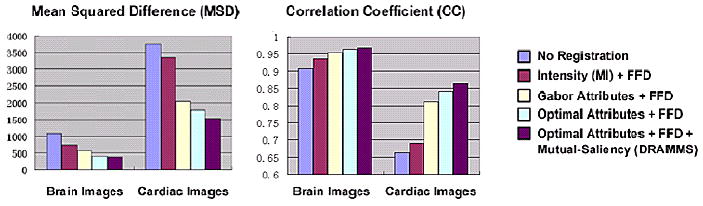
Quantitative evaluation of the registration accuracies of inter-subject brain and cardiac images, in terms of MSD and CC between registered and template images. The various parts of DRAMMS – feature extraction, feature selection, mutual-saliency weighting – are added into the experiment sequentially. As a result, this figure shows that each of DRAMMS' components provides additive improvement over MI-based FFD.
4.3. Atlas Construction
Our third set of experiments consists of atlas construction of human brain images. Fig. 13 shows 30 randomly selected brain MR images used for constructing a atlas. Each brain image is registered (in 3D) to the template (outlined by the red box), and then the warped images are averaged to form the atlas. The constructed atlases are shown in Fig. 14, from there DRAMMS is observed to result in sharper average, indicative of higher registration accuracy on average. Differences between the constructed atlases and the template image are further visualized for the central slice, as shown in the top row in Fig. 15. Also shown in Fig. 15 (bottom row) is the voxel-wise standard deviation among all warped images, by affine, MI-based FFD and DRAMMS methods, respectively. The smaller difference with the template in the top row and the smaller standard deviation among all warped images in the bottom row indicate the accuracy and the consistency of DRAMMS method over MI-based FFD. Fig. 16 shows mean squared difference (MSD), correlation coefficient (CC), and errors against expert-defined landmarks, between each warped subject image and the template image, by three registration methods, respectively. We specially emphasize Fig. 16(c), where DRAMMS recovers voxel correspondences closer to expert-defined locations in each single pair-wise case compared with MI-FFD method.
Figure 13.

The middle slices of the 30 randomly selected brain images used for constructing the atlas. The one in the bottom right is chosen as template image and is outlined by a red box.
Figure 14.

Brain atlases obtained from the randomly selected 30 images in Fig. 13. (a) Template, the same as the one in the red box in Fig. 13; (b) Atlas by affine registration; (c) Atlas obtained by MI-based FFD registration; (d) Atlas obtained by DRAMMS. The sharper average in (d) indicates higher registration accuracy for DRAMMS on average.
Figure 15.

Further comparison of affine, MI-based FFD and DRAMMS registration algorithms in atlas construction. (a1-c1) The difference image (=atlas-template) obtained from these three registration methods; (a2-c2) The standard deviation among all the warped images, by these registration methods, respectively. Smaller difference and smaller standard deviation indicate the accuracy and consistency of DRAMMS.
Figure 16.

Quantitative comparison of registration methods for each subject. (a) The mean squared difference (MSD) between warped image and the template for all foreground voxels. (b) The correlation coefficient between warped image and the template. (c) The errors (in voxels) against manually-defined landmark correspondences.
4.4. Multi-modality Registration
Our fourth set of experiments is on some fairly challenging multi-modality registration tasks. Normally, mutual information method is used for multi-modality registrations, as long as intensity distributions from the two images follow consistent relationship. However, when this assumption of consistent relationship in intensity distributions is violated, mutual information based methods are usually severally challenged. The registration between histological and MR images shown in Fig. 17 is one such case.
Figure 17.

Multi-modality registration between (a) histological and (b) MR images of the same prostate. Crosses of the same color denote the same spatial locations in all images, in order to better visualize the registration accuracy. Circles of the same colors roughly denote the corresponding regions, which are used to demonstrate the lack of consistent relationship in their intensity distributions.
For a brief background, histological images are usually taken in the ex vivo environment, by physically sectioning an organ into slices and examining the pathology of those slices under microscopy. Because of the ability to reveal pathologically authenticated ground truth for lesions and tumor, it is often of research interest to map ground truth from histological images to in vivo MR images of the same organ, so as to help doctors better understand the MR signal characteristics of lesions and tumor ??.
Specifically, histology-MRI registration is challenged by the fact that one image is from ex vivo whereas the other comes from in vivo, therefore, histological and MR images do not follow consistent relationship in their intensity distributions. For instance, in Fig. 17, we can observe dark regions corresponding to dark regions across images (blue circle), white regions corresponding to white regions across images (blue circles), but also dark regions corresponding to white regions (purple circles). Actually, the challenges in histology-MRI registration is far more several than in CT-MRI registration, because unlike CT-MRI case, where both are in vivo modalities, the ex vivo histological image and in vivo MR image have more drastic contrast differences and resolution differences, causing some structures clearly present in one image but almost invisible in the other. In this case, mutual information methods tend to be challenged, as demonstrated in a number of studies [Pitiot et al., 2006; Meyer et al., 2006; Dauguet et al., 2007]. To make things worse, tears/cuts often appear in the histological images, causing partial loss of correspondences. In Fig. 17, crosses of the same color have been placed at the same spatial locations in sub-figure (b), MR image, and (d) the warped histological image by DRAMMS, in order to visually reveal whether the anatomical structures have been successfully aligned. Compared with the artificial results obtained by MI-based FFD, DRAMMS leads to a smooth deformation field that better aligns tumor and other complicated structures.
5. Discussion
In this paper, a general purpose registration method named DRAMMS is presented. DRAMMS characterizes each voxel by an optimized multi-scale and multi-orientation Gabor attribute vector, therefore increases distinctiveness of each voxel and reduces the matching ambiguity. A second feature is that DRAMMS assigns continuously-valued weights for each voxel, based on a mutual-saliency measure that evaluates whether this voxel is capable of establishing reliable (unique) correspondences. With the assistance of this mutual-saliency weighting mechanism, the registration relies more on regions that can have reliable correspondences across images, and is therefore capable of reducing the negative impact caused by missing data and/or partial loss of correspondences. Experiments in simulated images, across-subject images and multi-modality images from human brain, heart and prostate have demonstrated the general applicability and registration accuracy of DRAMMS.
In the following, we will first discuss, in Sub-section 5.1, how DRAMMS bridges the gap between the two main categories of registration methods in the literature – voxel-wise methods and landmark/feature-based methods. Then, we will discuss the important issues in each of DRAMMS components – attribute extraction is discussed in Sub-section 5.2, attribute selection is discussed in Sub-section 5.3 and mutual-saliency weighting is discussed in Sub-section 5.4. In the end, we will discuss the difference between DRAMMS and a closely-related work HAMMER [Shen and Davatzikos, 2003] in Sub-section 5.5 and conclude the paper in Sub-section 5.6.
5.1. DRAMMS as a Bridge between Voxel-wise and Landmark/feature-based Methods
The two components in DRAMMS can be regarded as bridges between the traditional voxel-wise methods and the landmark/feature-based methods in two respects. This is listed in Table 2.
Table 2.
List of how DRAMMS bridges the gap between voxel-wise and landmark/feature-based registration methods.
| Voxel-wise | Landmark/feature-based | DRAMMS | |
|---|---|---|---|
| Voxel Characterization | Intensity | Task-specific attributes | Optimal Gabor attributes |
| (generally applicable to various tasks, but not distinctive for voxels) | (distinctive for voxels, but not generally applicable to various tasks) | (generally applicable to various tasks, and distinctive for voxels) | |
| Spatial Adaptivity (Voxel Utilization) | Not adaptive | Binarily adaptive | Continuously Adaptive |
| (Weight ≡ 1 for all voxels) | (Weight=1 for landmarks/features and 0 otherwise) | (Weighting voxels continuously by mutual-saliency measure) | |
5.2. Discussion on Attribute Extraction
Gabor attributes are used in the DRAMMS framework because of the three reasons mentioned in Section 2.2.1: general applicability; suitability in single- and multi-modality registration; and the multi-scale and multi-orientation nature.
When using Gabor filter banks, the number of scales, number of orientations, and the frequency range to be covered should all be carefully tuned. Ineffectively setting these parameters would unnecessarily introduce large redundancy among the attributes extracted, increasing the computational burden and decreasing the distinctiveness of attribute description. In this paper, we have adopted the parameter settings developed by [Manjunath and Ma, 1996], which have found success applications in numerous studies including [Zhan and Shen, 2006]. In particular, the number of scales is set at M = 4 and the number of orientations is set at N = 6, the highest frequency is set at 0.4Hz, the lowest frequency at 0.05Hz, and the size of the Gaussian envelope dependent on the highest frequency by a fixed relationship specified in equation 1 of their paper. Fig. 18 highlights the differences in the consequent similarity maps between adopting their set of parameters (sub-figures b, c, d, e) and adopting a random set of parameters (sub-figures b′, c′, d′, e′).
Figure 18.

Different similarity maps when using different parameter settings in Gabor filter banks for attribute extraction. All similarity maps are calculated between a cross point and all other points in the same image. (b-e) are similarity maps resulted from using Gabor parameters suggested in [Manjunath and Ma, 1996], while counterparts (b′-e′) are resulted from using a random set of Gabor parameters. This figure highlights the importance of adopting the right set of Gabor parameters.
There are, of course, other texture and geometric attributes that can easily fit into the framework of DRAMMS. Other options include gray-level cooccurrence matrix (GLCM) attributes [Haralick, 1979], spin image attributes [Lazebnik et al., 2005], RIFT (rotation-invariant feature transform) attributes [Lazebnik et al., 2005] and fractal attributes [Lopes and Betrouni, 2009]. Although Gabor attributes are believed to be a proper choice because of the three merits listed in Section 2.2.1 and because of the experimental comparison in Fig. 8, a rigorous comparative study among all these attributes in the registration context should be of interest. Such a study is a non-trivial task, as it requires a large number of images to be registered, requires objective evaluation of registration accuracies, which is difficult, and ideally, requires quantitative analysis of the number and the depth of local minima in the cost function as a result of different attributes or their different combinations. We mark such a study as one of our future research directions.
5.3. Discussion on Attribute Selection
Although the overlaps/redundancies among Gabor filter banks can be largely reduced by carefully choosing a set of parameters in the very beginning, the redundancy will almost never vanish completely, simply because of the non-orthogonal nature among Gabor filters. Therefore, the attribute selection module is needed to further reduce information redundancy and also computational burden.
Key to the selection of attributes is the quantification of matching reliability and matching uniqueness, especially the latter. Quantification of matching uniqueness (by mutual-saliency) enables us to find voxels and attributes components that not only render true correspondences similar, but more importantly, render them uniquely similar, meaning similar to each other and not similar to anything else in the neighborhood.
Another nice feature of the attribute selection part is that no a priori knowledge is required. It is designed to take no other input except the two input images being registered, therefore keeping DRAMMS a general-purpose method.
Nevertheless, if a priori knowledge is given, DRAMMS framework can be readily extended to incorporate it without much efforts. For instance, if there are a number of anatomically corresponding voxels given by experts, then we can directly rely on them to select the optimal attributes and simply skip the step of selecting the training voxel pairs, as long as the expert-defined voxel pairs are 1) mutually-salient, 2) representative of anatomic/geometric context in images and 3) ideally, spatially distributed. A priori knowledge can be also obtained if registration is restricted to a specific type of images (e.g. human brain MRI registration). In this case, a common set of optimal attributes can be learned when registering a large set of such images. This should provide considerable speedup of the algorithm for some common registration tasks.
5.4. Discussion on Mutual-Saliency Weighting
The mutual-saliency value is automatically derived to reflect whether the matching between a pair of voxels is reliable (unique) in the neighborhood. Since saliency is measured individually in one image and matching uniqueness is measured across images, neither single saliency or double saliency necessarily lead to matching uniqueness. That is the motivation for developing mutual-saliency, which directly measure uniqueness across images. Therefore, it can more effectively capture regions/voxels useful for registration and regions/voxels having difficulties establishing correspondences.
The mutual-saliency map seems to be most helpful under circumstances of missing data, or partial loss of correspondences. A typical example is the image cuts/stitches when registering histological images with MR images (like in Figs. 11 and 17). Another typical example is the lesions/tumors when registering diseased images with normal images (e.g. Fig. 1). In these cases, existing methods without using mutual-saliency weighting tend to over-aggressively match structures that should not have been corresponding to each other. Although the over-aggressive matching usually lead to smaller residual (like in Fig. 11(c)), they are not desirable because of the artificial images after registration and because of the often convoluted deformations. In contrast, the mutual-saliency maps guide registration to match well the structures that should have been matched, and leave the structures that have difficulty finding correspondences almost untouched. When the negative impact of the loss of correspondence is reduced (such as demonstrated in Fig. ??), the registered image is more anatomically meaningful (like in Fig. 11(f)), and the relative larger intensity residual becomes a right descriptor to encode the missing data.
It should be noted that the mutual-saliency calculation itself is usually computationally costly, because it checks voxel-wise similarities in a neighborhood for each individual voxel, and on top of that, because all these similarities are calculated from high-dimensional attribute vectors. The computational cost of mutual-saliency map can be observed in Table 1, where incorporating mutual-saliency in the registration will usually cost considerably more computational time. Therefore, for those registration tasks that do not involve missing data or loss of correspondence, the mutual-saliency component can be probably dropped, with noticeable speedup and moderate decrease of registration accuracy.
5.5. Differences between DRAMMS and HAMMER
We refer to HAMMER registration algorithm [Shen and Davatzikos, 2003] as the one closest to DRAMMS. HAMMER algorithm pioneers the attribute-matching concept, where it extracts geometric-moment-invariant (GMI) attributes, tissue membership attributes and boundary/edge attributes for brain image registrations. We point out the following differences between the two methods:
Spatial adaptivity is different. HAMMER is essentially a landmark/feature-based method and therefore may inherit some challenges that are inherent to landmark/feature-based methods. DRAMMS is a voxel-wise method with mutual-saliency weightings on each voxel.
Suitable application is different. HAMMER is specifically designed for normal brain image registration, as the attributes of tissue membership require segmentation of brain tissue types prior to registration. DRAMMS is a general-purpose method, as the Gabor attribute extraction can be generally applied to any images, regardless of modalities and contents. DRAMMS can even apply to registration with missing data and partial loss of correspondences.
Deformation mechanism is different. HAMMER has its own deformation mechanism, where the movement of one landmark/feature voxel will guide the movement of neighboring voxels in a Gaussian kernel. The deformation mechanism is usually aggressive and, in some cases, not diffeomorphic. DRAMMS is based on diffeomorphic FFD model that guarantees diffeomorphism.
In this paper, DRAMMS is only compared with other general-purpose methods, and it will be interesting to compare with those specific-purpose methods including HAMMER in future studies, to better establish registration accuracies.
5.6. Conclusion
In summary, a general-purpose image registration method named “DRAMMS” has been presented in this paper. In DRAMMS, more distinctive characterization of voxels leads to reduced matching ambiguities, and more spatially adaptive utilization of imaging data leads to robustness with regard to missing data or partial loss of correspondences. Future work includes comparing different texture/geometric attributes in the framework, better understanding the effect of mutual-saliency in registration scenarios with outliers, and more extensively comparing our method with existing ones in various registration tasks.
Acknowledgments
The authors would like to thank the reviewers for their careful reviews and their constructive comments and suggestions, which help improve the quality of this paper.
Footnotes
Publisher's Disclaimer: This is a PDF file of an unedited manuscript that has been accepted for publication. As a service to our customers we are providing this early version of the manuscript. The manuscript will undergo copyediting, typesetting, and review of the resulting proof before it is published in its final citable form. Please note that during the production process errors may be discovered which could affect the content, and all legal disclaimers that apply to the journal pertain.
References
- Anandan P. A computational framework and an algorithm for the measurement of visual motion. International Journal of Computer Vision. 1989;2:283–310. [Google Scholar]
- Ashburner J. A fast diffeomorphic image registration algorithm. NeuroImage. 2007;38(1):95–113. doi: 10.1016/j.neuroimage.2007.07.007. [DOI] [PubMed] [Google Scholar]
- Bai W, Brady M. Regularized b-spline deformable registration for respiratory motion correction in PET images. Physics in Medicine and Biology. 2009;54(9):2719–2736. doi: 10.1088/0031-9155/54/9/008. [DOI] [PubMed] [Google Scholar]
- Bond S, Brady J. Non-rigid registration for colorectal cancer MR images. Computer Vision for Biomedical Image Applications (CVBIA) 2005:399–408. [Google Scholar]
- Bookstein FL. Principal warps: thin-plate splines and the decomposition of deformations. Pattern Analysis and Machine Intelligence, IEEE Transactions on. 1989;11(6):567–585. [Google Scholar]
- Chen X, Brady M, Lo JLC, Moore N. Simultaneous segmentation and registration of contrast-enhanced breast mri. Information Processing in Medical Imaging (IPMI) 2005:126–137. doi: 10.1007/11505730_11. [DOI] [PubMed] [Google Scholar]
- Choi Y, Lee Y. Injectivity conditions of 2d and 3d uniform cubic b-spline functions. Graphical Models. 2000;62(6):411–427. [Google Scholar]
- Christensen GE, Rabbitt RD, Miller MI. 3d brain mapping using a deformable neuroanatomy. Physics in Medicine and Biology. 1994;39(3):609–618. doi: 10.1088/0031-9155/39/3/022. [DOI] [PubMed] [Google Scholar]
- Chui H, Rangarajan A. A new point matching algorithm for non-rigid registration. Computer Vision and Image Understanding. 2003;89:114–141. [Google Scholar]
- Collins DL, Neelin P, Peters TM, Evans AC. Automatic 3d intersubject registration of MR volumetric data in standardized talairach space. Journal of Computer Assisted Tomography. 1994;18(2):192–205. [PubMed] [Google Scholar]
- Crum WR, Hartkens T, Hill DL. Non-rigid image registration: theory and practice. The British Journal of Radiology. 2004;77(2):140–153. doi: 10.1259/bjr/25329214. [DOI] [PubMed] [Google Scholar]
- Csapo I, Holland C, Guttmann C. Image registration framework for large-scale longitudinal MRI data sets: strategy and validation. Magnetic Resonance Imaging. 2007;25(6):889–893. doi: 10.1016/j.mri.2007.03.004. [DOI] [PubMed] [Google Scholar]
- D'Agostino E, Maes F, Vandermeulen D, Suetens P. A viscous fluid model for multimodal non-rigid image registration using mutual information. Medical Image Analysis. 2003;7(4):565–575. doi: 10.1016/s1361-8415(03)00039-2. [DOI] [PubMed] [Google Scholar]
- Dauguet J, Delzescaux T, Conde F, Mangin J, Ayache N, Hantraye P, Frouin V. Three-dimensional reconstruction of stained histological slices and 3d non-linear registration with in-vivo mri for whole baboon brain. Journal of Neur. Methods. 2007;164:191–204. doi: 10.1016/j.jneumeth.2007.04.017. [DOI] [PubMed] [Google Scholar]
- Davatzikos C, Prince J, Bryan R. Image registration based on boundary mapping. IEEE Transactions on Medical Imaging. 1996;15(1):112–115. doi: 10.1109/42.481446. [DOI] [PubMed] [Google Scholar]
- Duncan J, Owen R, Staib L, Anandan P. Measurement of non-rigid motion using contour shape descriptors. Computer Vision and Pattern Recognition (CVPR) 1991:318–324. [Google Scholar]
- Elbakary M, Sundareshan M. Accurate representation of local frequency using a computationally efficient gabor filter fusion approach with application to image registration. Pattern Recognition Letters. 2005;26(14):2164–2173. [Google Scholar]
- Ellingsen L, Prince J. Mjolnir: Extending HAMMER using a diffusion transformation model and histogramequalization for deformable image registration. International Journal of Biomedical Imaging. 2009;2009:18. doi: 10.1155/2009/281615. Article ID 281615. [DOI] [PMC free article] [PubMed] [Google Scholar]
- Fan Y, Shen D, Gur RC, Gur RE, Davatzikos C. COMPARE: Classification of morphological patterns using adaptive regional elements. Medical Imaging, IEEE Transactions on. 2007;26(1):93–105. doi: 10.1109/TMI.2006.886812. [DOI] [PubMed] [Google Scholar]
- Foroughi P, Abolmaesumi P. Elastic registration of 3d ultrasound images. Medical Image Computing and Computer-Assisted Intervention (MICCAI) 2005:83–90. doi: 10.1007/11566465_11. [DOI] [PubMed] [Google Scholar]
- Friston KJ, Ashburner J, Frith CD, Poline JB, Heather JD, Frackowiak RSJ. Spatial registration and normalization of images. Human Brain Mapping. 1995;3(3):165–189. [Google Scholar]
- Gee J, Barillot C, Le Briquer L, Haynor D, Bajcsy R. Proc SPIE, Visualization in Biomedical Computing. 1994. Matching structural images of the human brain using statistical and geometrical image features; pp. 191–204. [Google Scholar]
- Gee JC, Reivich M, Bajcsy R. Elastically deforming 3d atlas to match anatomical brain images. Journal of Computer Assisted Tomography. 1993;17(2):225–236. doi: 10.1097/00004728-199303000-00011. [DOI] [PubMed] [Google Scholar]
- Geng X, Christensen GE, Gu H, Ross TJ, Yang Y. Implicit reference-based group-wise image registration and its application to structural and functional mri. NeuroImage. 2009;47(4):1341–1351. doi: 10.1016/j.neuroimage.2009.04.024. [DOI] [PMC free article] [PubMed] [Google Scholar]
- Gering DT, Nabavi A, Kikinis R, Hata N, O'Donnell LJ, Grimson WE, Jolesz FA, Black PM, Wells WM. An integrated visualization system for surgical planning and guidance using image fusion and an open mr. Journal of Magnetic Resonance Imaging. 2001;13(6):967–975. doi: 10.1002/jmri.1139. [DOI] [PubMed] [Google Scholar]
- Glocker B, Komodakis N, Tziritas G, Navab N, Paragios N. Dense image registration through MRFs and efficient linear programming. Medical Image Analysis. 2008;12(6):731–741. doi: 10.1016/j.media.2008.03.006. [DOI] [PubMed] [Google Scholar]
- Guyon I, Elisseeff A. An introduction to variable and feature selection. Journal of Machine Learning Research. 2003;3:1157–1182. [Google Scholar]
- Haralick RM. Statistical and structural approaches to texture. Proceedings of the IEEE. 1979;67(5):786–804. [Google Scholar]
- Hata N, Dohi T, Warfield S, Wells W, Kikinis R, Jolesz F. Multimodality deformable registration of pre- and intraoperative images for MRI-guided brain surgery. International Conference on Medical Image Computing and Computer Assisted Intervention (MICCAI); 1998. pp. 1067–1074. [Google Scholar]
- Hill DL, Batchelor PG, Holden M, Hawkes DJ. Medical image registration. Physics in Medicine and Biology. 2001;46(3):1–45. doi: 10.1088/0031-9155/46/3/201. [DOI] [PubMed] [Google Scholar]
- Holden M. A review of geometric transformations for nonrigid body registration. Medical Imaging, IEEE Transactions on. 2008;27(1):111–128. doi: 10.1109/TMI.2007.904691. [DOI] [PubMed] [Google Scholar]
- Huang X, Sun Y, Metaxas D, Sauer F, Xu C. Hybrid image registration based on configural matching of scale-invariant salient region features. Proceedings of the 2004 Conference on Computer Vision and Pattern Recognition Workshop (CVPRW'04); 2004. [Google Scholar]
- Jain AK, Farrokhnia F. Unsupervised texture segmentation using gabor filters. Pattern Recognition. 1991;24(12):1167–1186. [Google Scholar]
- Jian B, Vemuri B, Marroquin J. Robust nonrigid multimodal image registration using local frequency maps. Information Processing in Medical Imaging (IPMI) 2005:504–515. doi: 10.1007/11505730_42. [DOI] [PMC free article] [PubMed] [Google Scholar]
- Joshi S, Davis B, Jomier M, Gerig G. Unbiased diffeomorphic atlas construction for computational anatomy. NeuroImage. 2004;23(1):151–160. doi: 10.1016/j.neuroimage.2004.07.068. [DOI] [PubMed] [Google Scholar]
- Joshi SC, Miller MI. Landmark matching via large deformation diffeomorphisms. Image Processing, IEEE Transactions on. 2000;9(8):1357–1370. doi: 10.1109/83.855431. [DOI] [PubMed] [Google Scholar]
- Kadir T, Brady M. Saliency, scale and image description. International Journal of Computer Vision. 2001;45(2):83–105. [Google Scholar]
- Kamarainen J. PhD thesis. Lappeenranta University of Technology; Finland: 2003. Feature extraction using gabor filters. [Google Scholar]
- Komodakis N, Tziritas G, Paragios N. Performance vs computational efficiency for optimizing single and dynamic mrfs: Setting the state of the art with primal-dual strategies. Computer Vision and Image Understanding. 2008;112(1):14–29. [Google Scholar]
- Kybic J, Unser M. Fast parametric elastic image registration. Image Processing, IEEE Transactions on. 2003;12(11):1427–1442. doi: 10.1109/TIP.2003.813139. [DOI] [PubMed] [Google Scholar]
- Lawes I, Barrick T, Murugam V, Spierings N, Evans D, Song M, Clark C. Atlas-based segmentation of white matter tracts of the human brain using diffusion tensor tractography and comparison with classical dissection. NeuroImage. 2008;39(1):62–79. doi: 10.1016/j.neuroimage.2007.06.041. [DOI] [PubMed] [Google Scholar]
- Lazebnik S, Schmid C, Ponce J. A sparse texture representation using local affine regions. Pattern Analysis and Machine Intelligence, IEEE Transactions on. 2005;27(8):1265–1278. doi: 10.1109/TPAMI.2005.151. [DOI] [PubMed] [Google Scholar]
- Leow A, Yanovsky I, Chiang M, Lee A, Klunder A, Lu A, Becker J, Davis S, Toga A, Thompson P. Statistical properties of jacobian maps and the realization of unbiased large-deformation nonlinear image registration. IEEE Transactions on Medical Imaging. 2007;26(6):822–832. doi: 10.1109/TMI.2007.892646. [DOI] [PubMed] [Google Scholar]
- Lester H, Arridge S. A survey of hierarchical non-linear medical image registration. Pattern Recognition. 1999;32(1):129–149. [Google Scholar]
- Li G, Guo L, Liu T. Deformation invariant attribute vector for deformable registration of longitudinal brain MR images. Computerized Medical Imaging and Graphics. 2009;33(5):273–297. doi: 10.1016/j.compmedimag.2009.03.004. [DOI] [PMC free article] [PubMed] [Google Scholar]
- Liao S, Chung A. Non-rigid image registration with uniform spherical structure patterns. Information Processing in Medical Imaging (IPMI) 2009:163–175. doi: 10.1007/978-3-642-02498-6_14. [DOI] [PubMed] [Google Scholar]
- Ling H, Jacobs D. Deformation invariant image matching. The Tenth International Conference in Computer Vision (ICCV); Beijing, China. 2005. [Google Scholar]
- Liu J, Vemuri BC, Marroquin JL. Local frequency representations for robust multimodal image registration. IEEE Transactions on Medical Imaging. 2002;21(5):462–469. doi: 10.1109/TMI.2002.1009382. [DOI] [PubMed] [Google Scholar]
- Liu T, Shen D, Davatzikos C. Deformable registration of cortical structures via hybrid volumetric and surface warping. NeuroImage. 2004;22(4):1790–1801. doi: 10.1016/j.neuroimage.2004.04.020. [DOI] [PubMed] [Google Scholar]
- Lopes R, Betrouni N. Fractal and multifractal analysis: A review. Medical Image Analysis. 2009;13(4):634–649. doi: 10.1016/j.media.2009.05.003. [DOI] [PubMed] [Google Scholar]
- Luan H, Qi F, Xue Z, Chen L, Shen D. Multimodality image registration by maximization of quantitativecqualitative measure of mutual information. Pattern Recognition. 2008;41(1):285–298. [Google Scholar]
- Maes F, Collignon A, Vandermeulen D, Marchal G, Suetens P. Multimodality image registration by maximization of mutual information. Medical Imaging, IEEE Transactions on. 1997;16(2):187–198. doi: 10.1109/42.563664. [DOI] [PubMed] [Google Scholar]
- Mahapatra D, Sun Y. Registration of dynamic renal MR images using neurobiological model of saliency. IEEE International Symposium on Biomedical Imaging (ISBI); 2008. pp. 1119–1122. [Google Scholar]
- Maintz JBA, Viergever MA. A survey of medical image registration. Medical Image Analysis. 1998;2(1):1–36. doi: 10.1016/s1361-8415(01)80026-8. [DOI] [PubMed] [Google Scholar]
- Manjunath BS, Ma W. Texture features for browsing and retrieval of image data. IEEE Transactions on Pattern Analysis and Machine Intelligence. 1996;18(8):837–842. [Google Scholar]
- McAuliffe M, Lalonde F, McGarry D, Gandler W, Csaky K, Trus B. Proc 14th IEEEComputer-Based Medical Systems. 2001. Medical image processing, analysis and visualization in clinical research; pp. 381–386. [Google Scholar]
- McEachen J, Duncan JS. Shape-based tracking of left ventricular wall motion. Medical Imaging, IEEE Transactions on. 1997;16(3):270–283. doi: 10.1109/42.585761. [DOI] [PubMed] [Google Scholar]
- Meyer C, Boes J, Kim B, Bland P, Zasadny K, Kison P, Koral K, Frey K, Wahl R. Demonstration of accuracy and clinical versatility of mutual information for automatic multimodality image fusion using affine and thin-plate spline warped geometric deformations. Medical Image Analysis. 1997;1(3):195–206. doi: 10.1016/s1361-8415(97)85010-4. [DOI] [PubMed] [Google Scholar]
- Meyer C, Moffat B, Kuszpit K, Bland P, Mckeever P, Johnson T, Chenevert T, Rehemtulla A, Ross B. A methodology for registration of a histological slide and in vivo MRI volume based on optimizing mutual information. Molecular Imaging. 2006;5(1):16–23. [PMC free article] [PubMed] [Google Scholar]
- Munoz-Moreno E, Cardenes-Almeida R, Martin-Fernandez M. Review of techniques for registration of diffusion tensor imaging. Tensors in Image Processing and Computer Vision. 2009:273–297. [Google Scholar]
- Muratore D, Russ J, Dawant B, Galloway RJ. Three-dimensional image registration of phantom vertebrae for image-guided surgery: A preliminary study. Comuter Aided Surgey. 2003;7(6):342–352. doi: 10.1002/igs.10055. [DOI] [PubMed] [Google Scholar]
- Ou Y, Davatzikos C. DRAMMS: Deformable registration via attribute matching and mutual-saliency weighting. 2009:50–62. doi: 10.1007/978-3-642-02498-6_5. [DOI] [PubMed] [Google Scholar]
- Ou Y, Shen D, Feldman M, Tomaszewski J, Davatzikos C. Non-rigid registration between histological and MR images of the prostate: A joint segmentation and registration framework. 2009a:125–132. [Google Scholar]
- Ou Y, Shen D, Zeng J, Sun L, Moul J, Davatzikos C. Sampling the spatial patterns of cancer: Optimized biopsy procedures for estimating prostate cancer volume and gleason score. Medical Image Analysis. 2009b;13(4):609–620. doi: 10.1016/j.media.2009.05.002. [DOI] [PMC free article] [PubMed] [Google Scholar]
- Pitiot A, Bardinet E, Thompson P, Malandain G. Piecewise affine registration of biological images for volume reconstruction. Medical Image Analysis. 2006;10(3):465–483. doi: 10.1016/j.media.2005.03.008. [DOI] [PubMed] [Google Scholar]
- Pluim JPW, Maintz JBA, Viergever MA. Mutual-information-based registration of medical images: a survey. Medical Imaging, IEEE Transactions on. 2003;22(8):986–1004. doi: 10.1109/TMI.2003.815867. [DOI] [PubMed] [Google Scholar]
- Pohl KM, Fisher J, Grimson E, Kininis R, Wells WM. A bayesian model for joint segmentation and registration. NeuroImage. 2006;31:228–239. doi: 10.1016/j.neuroimage.2005.11.044. [DOI] [PubMed] [Google Scholar]
- Prastawa M, Gilmore JH, Lin W, Gerig G. Automatic segmentation of MR images of the developing newborn brain. Medical Image Analysis. 2005;9(5):457–466. doi: 10.1016/j.media.2005.05.007. [DOI] [PubMed] [Google Scholar]
- Rohr K, Stiehl HS, Sprengel R, Buzug TM, Weese J, Kuhn MH. Landmark-based elastic registration using approximating thin-plate splines. Medical Imaging, IEEE Transactions on. 2001;20(6):526–534. doi: 10.1109/42.929618. [DOI] [PubMed] [Google Scholar]
- Rueckert D, Aljabar P, Heckemann RA, Hajnal JV, Hammers A. Diffeomorphic registration using b-splines. Medical Image Computing and Computer-Assisted Intervention (MICCAI) 2006:702–709. doi: 10.1007/11866763_86. [DOI] [PubMed] [Google Scholar]
- Rueckert D, Sonoda LI, Hayes C, Hill DL, Leach MO, Hawkes DJ. Nonrigid registration using free-form deformations: application to breast MR images. IEEE Transactions on Medical Imaging. 1999 August;18(8):712–721. doi: 10.1109/42.796284. [DOI] [PubMed] [Google Scholar]
- Shen D. Image registration by local histogram matching. Pattern Recognition. 2007;40(4):1161–1172. [Google Scholar]
- Shen D, Davatzikos C. HAMMER: hierarchical attribute matching mechanism for elastic registration. Medical Imaging, IEEE Transactions on. 2003 February;21(11):1421–1439. doi: 10.1109/TMI.2002.803111. [DOI] [PubMed] [Google Scholar]
- Shen D, Davatzikos C. Measuring temporal morphological changes robustly in brain mr images via 4-dimensional template warping. NeuroImage. 2004;21(4):1508–1517. doi: 10.1016/j.neuroimage.2003.12.015. [DOI] [PubMed] [Google Scholar]
- Shen D, Herskovits E, Davatzikos C. An adaptive-focus statistical shape model for segmentation and shape modeling of 3-d brain structures. IEEE Transactions on Medical Imaging. 2001;20(4):257–270. doi: 10.1109/42.921475. [DOI] [PubMed] [Google Scholar]
- Shi P, Sinusas AJ, Constable RT, Ritman E, Duncan JS. Point-tracked quantitative analysis of left ventricular surface motion from 3-d image sequences. IEEE Transactions on Medical Imaging. 2000;19(1):36–50. doi: 10.1109/42.832958. [DOI] [PubMed] [Google Scholar]
- Sotiras A, Komodakis N, Glocker B, Paragios N. Graphical models and deformable diffeomorphic population registration using global and local metrics. International Conference on Medical Image Computing and Computer Assisted Intervention (MICCAI); 2009. [DOI] [PubMed] [Google Scholar]
- Sundar H, Litt H, Shen D. Estimating myocardial motion by 4d image warping. Pattern Recognition. 2009;42(11):2514–2526. doi: 10.1016/j.patcog.2009.04.022. [DOI] [PMC free article] [PubMed] [Google Scholar]
- Thirion JP. Image matching as a diffusion process: An analogy with maxwell's demons. Medical Image Analysis. 1998;2(3):243–260. doi: 10.1016/s1361-8415(98)80022-4. [DOI] [PubMed] [Google Scholar]
- Thompson P, Toga AW. A surface-based technique for warping three-dimensional images of the brain. Medical Imaging, IEEE Transactions on. 1996;15(4):402–417. doi: 10.1109/42.511745. [DOI] [PubMed] [Google Scholar]
- Thompson PM, Apostolova LG. Computational anatomical methods as applied to ageing and dementia. The British journal of radiology. 2007;80:78–91. doi: 10.1259/BJR/20005470. [DOI] [PubMed] [Google Scholar]
- Vercauteren T, Pennec X, Perchant A, Ayache N. Non-parametric diffeomorphic image registration with the demons algorithm. International Conference on Medical Image Computing and Computer Assisted Intervention (MICCAI); 2007. pp. 319–326. [DOI] [PubMed] [Google Scholar]
- Vercauteren T, Pennec X, Perchant A, Ayache N. Diffeomorphic demons: Efficient non-parametric image registration. NeuroImage. 2009;45(1):S61–S72. doi: 10.1016/j.neuroimage.2008.10.040. [DOI] [PubMed] [Google Scholar]
- Verma R, Davatzikos C. Matching of diffusion tensor images using gabor features. IEEE International Symposium on Biomedical Imaging (ISBI); 2004. pp. 396–399. [Google Scholar]
- Verma R, Zacharaki E, Ou Y, Cai H, Chawla S, Lee S, Melhem E, Wolf R, Davatzikos C. Multiparametric tissue characterization of brain neoplasms and their recurrence using pattern classification of mr images. Acadmic Radiology. 2008;15(8):966–977. doi: 10.1016/j.acra.2008.01.029. [DOI] [PMC free article] [PubMed] [Google Scholar]
- Wang F, Vemuri BC, Eisenschenk SJ. Joint registration and segmentation from brain mri. Academic Radiology. 2006;13(9):1101–1111. doi: 10.1016/j.acra.2006.05.017. [DOI] [PMC free article] [PubMed] [Google Scholar]
- Wells W, Viola P, Atsumi H, Nakajima S, Kikinis R. Multi-modal volume registration by maximization of mutual information. Medical Image Analysis. 1996;1(1):35–51. doi: 10.1016/s1361-8415(01)80004-9. [DOI] [PubMed] [Google Scholar]
- Wu G, Qi F, Shen D. Learning-based deformable registration of MR brain images. IEEE Transactions on Medical Imaging. 2006;25(9):1145, 1157. doi: 10.1109/tmi.2006.879320. [DOI] [PubMed] [Google Scholar]
- Wu G, Qi F, Shen D. Learning best features and deformation statistics for hierarchical registration of MR brain images. Information Processing in Medical Imaging (IPMI) 2007:160–171. doi: 10.1007/978-3-540-73273-0_14. [DOI] [PubMed] [Google Scholar]
- Wyatt P, Nobel J. Map mrf joint segmentation and registration of medical images. Medical Image Analysis. 2003;7:539–552. doi: 10.1016/s1361-8415(03)00067-7. [DOI] [PubMed] [Google Scholar]
- Xing Y, Xue Z, Englander S, Schnall M, Shen D. Improving parenchyma segmentation by simultaneous estimation of tissue property t1 map and group-wise registration of inversion recovery mr breast images. Medical Image Computing and Computer-Assisted Intervention (MICCAI) 2008:342–350. doi: 10.1007/978-3-540-85988-8_41. [DOI] [PubMed] [Google Scholar]
- Xue Z, Long L, Antani S, Jeronimo J, Thoma G. Proceedings of SPIE Medical Imaging. 2009. Segmentation of mosaicism in cervicographic images using support vector machines. [Google Scholar]
- Xue Z, Shen D, Davatzikos C. Determining correspondence in 3-d MR brain images using attribute vectors as morphological signatures of voxels. IEEE Transactions on Medical Imaging. 2004;23(10):1276–1291. doi: 10.1109/TMI.2004.834616. [DOI] [PubMed] [Google Scholar]
- Xue Z, Shen D, Davatzikos C. CLASSIC: Consistent longitudinal alignment and segmentation for serial image computing. NeuroImage. 2006;30(2):388–399. doi: 10.1016/j.neuroimage.2005.09.054. [DOI] [PubMed] [Google Scholar]
- Xue Z, Wong KSW. Joint registration and segmentation of serial lung ct images in microendoscopy molecular image- guided therapy. Medical Imaging and Augmented Reality. 2008:12–20. doi: 10.1016/j.compmedimag.2009.05.007. [DOI] [PMC free article] [PubMed] [Google Scholar]
- Yang J, Blum RS, Williams J, Sun Y, Xu C. Non-rigid image registration using geometric features and local salient region features. IEEE Computer Society Conference on Computer Vision and Pattern Recognition (CVPR); 2006. pp. 825–832. [Google Scholar]
- Yang J, Shen D, Davatzikos C. Diffusion tensor image registration using tensor geometry and orientation features. Medical Image Computing and Computer-Assisted Intervention (MICCAI) 2008:905–913. doi: 10.1007/978-3-540-85990-1_109. [DOI] [PubMed] [Google Scholar]
- Yap P, Wu G, Zhu H, Lin W, Shen D. TIMER: Tensor image morphing for elastic registration. NeuroImage. 2009;47:549–563. doi: 10.1016/j.neuroimage.2009.04.055. [DOI] [PMC free article] [PubMed] [Google Scholar]
- Yezzi A, Zollei L, Kapur T. A variational framework for joint segmentation and registration. Mathematical Methods in Biomedical Image Analysis (MMBIA) 2001 doi: 10.1016/s1361-8415(03)00004-5. [DOI] [PubMed] [Google Scholar]
- Zacharaki E, Shen D, Lee S, Davatzikos C. Orbit: A multiresolution framework for deformable registration of brain tumor images. IEEE Transactions on Medical Imaging. 2008;27(8):1003–1017. doi: 10.1109/TMI.2008.916954. [DOI] [PMC free article] [PubMed] [Google Scholar]
- Zhan Y, Ou Y, Feldman M, Tomaszeweski J, Davatzikos C. Registering histologic and MR images of prostate for image-based cancer detection. Academic Radiology. 2007;14(11):1367–1381. doi: 10.1016/j.acra.2007.07.018. [DOI] [PMC free article] [PubMed] [Google Scholar]
- Zhan Y, Shen D. Deformable segmentation of 3d ultrasound prostate images using statistical texture matching method. IEEE Transactions on Medical Imaging. 2006;25:256–272. doi: 10.1109/TMI.2005.862744. [DOI] [PubMed] [Google Scholar]
- Zhang J, Liu Y. Cervical cancer detection using SVM based feature screening. Medical Image Computing and Computer Assisted Intervention (MICCAI) 2004:873–880. [Google Scholar]
- Zitova B, Flusser J. Image registration methods: a survey. Image and Vision Computing. 2003;21(11):977–1000. [Google Scholar]
- Zollei L, Learned-Miller E, Grimson E, Wells WI. Efficient population registration of 3d data. ICCV Workshop: Computer Vision for Biomedical Image Applications (CVBIA) 2005:291–301. [Google Scholar]
- Zuo C, Jiang A, Buff B, Mahon T, Wong T. Automatic motion correction for breast MR imaging. Radiology. 1996;198:903–906. doi: 10.1148/radiology.198.3.8628891. [DOI] [PubMed] [Google Scholar]