

Abstract
Nonlinear stochastic dynamical systems are widely used to model systems across the sciences and engineering. Such models are natural to formulate and can be analyzed mathematically and numerically. However, difficulties associated with inference from time-series data about unknown parameters in these models have been a constraint on their application. We present a new method that makes maximum likelihood estimation feasible for partially-observed nonlinear stochastic dynamical systems (also known as state-space models) where this was not previously the case. The method is based on a sequence of filtering operations which are shown to converge to a maximum likelihood parameter estimate. We make use of recent advances in nonlinear filtering in the implementation of the algorithm. We apply the method to the study of cholera in Bangladesh. We construct confidence intervals, perform residual analysis, and apply other diagnostics. Our analysis, based upon a model capturing the intrinsic nonlinear dynamics of the system, reveals some effects overlooked by previous studies.
Keywords: maximum likelihood, cholera, time series
State space models have applications in many areas, including signal processing (1), economics (2), cell biology (3), meteorology (4), ecology (5), neuroscience (6), and various others (7–9). Formally, a state space model is a partially observed Markov process. Real-world phenomena are often well modeled as Markov processes, constructed according to physical, chemical, or economic principles, about which one can make only noisy or incomplete observations.
It has been noted repeatedly (1, 10) that estimating parameters for state space models is simplest if the parameters are time-varying random variables that can be included in the state space. Estimation of parameters then becomes a matter of reconstructing unobserved random variables, and inference may proceed by using standard techniques for filtering and smoothing. This approach is of limited value if the true parameters are thought not to vary with time, or to vary as a function of measured covariates rather than as random variables. A major motivation for this work has been the observation that the particle filter (9–13) is a conceptually simple, flexible, and effective filtering technique for which the only major drawback was the lack of a readily applicable technique for likelihood maximization in the case of time-constant parameters. The contribution of this work is to show how time-varying parameter algorithms may be harnessed for use in inference in the fixed-parameter case. The key result, Theorem 1, shows that an appropriate limit of time-varying parameter models can be used to locate a maximum of the fixed-parameter likelihood. This result is then used as the basis for a procedure for finding maximum likelihood estimates for previously intractable models.
We use the method to further our understanding of the mechanisms of cholera transmission. Cholera is a disease endemic to India and Bangladesh that has recently become reestablished in Africa, south Asia, and South America (14). It is highly contagious, and the direct fecal–oral route of transmission is clearly important during epidemics. A slower transmission pathway, via an environmental reservoir of the pathogen, Vibrio cholerae, is also believed to be important, particularly in the initial phases of epidemics (15). The growth rate of V. cholerae depends strongly on water temperature and salinity, which can fluctuate markedly on both seasonal and interannual timescales (16, 17). Important climatic fluctuations, such as the El Niño Southern Oscillation (ENSO), affect temperature and salinity, and operate on a time scale comparable to that associated with loss of immunity (18, 19). Therefore, it is critical to disentangle the intrinsic dynamics associated with cholera transmission through the two main pathways and with loss of immunity, from the extrinsic forcing associated with climatic fluctuations (20).
We consider a model for cholera dynamics that is a continuous-time version of a discrete-time model considered by Koelle and Pascual (20), who in turn followed a discrete-time model for measles (21). Discrete-time models have some features that are accidents of the discretization; working in continuous time avoids this, and also allows inclusion of covariates measured at disparate time intervals. Maximum likelihood inference has various convenient asymptotic properties: it is efficient, standard errors are available based on the Hessian matrix, and likelihood can be compared between different models. The transformation-invariance of maximum likelihood estimates allows modeling at a natural scale. Non-likelihood approaches typically require a variance-stabilizing transformation of the data, which may confuse scientific interpretation of results. Some previous likelihood-based methods have been proposed (22–25). However, the fact that non-likelihood-based statistical criteria such as least square prediction error (26) or gradient matching (27) are commonly applied to ecological models of the sort considered here is evidence that likelihood-based methods continue to be difficult to apply. Recent advances in nonlinear analysis have brought to the fore the need for improved statistical methods for dealing with continuous-time models with measurement error and covariates (28).
Maximum Likelihood via Iterated Filtering
A state space model consists of an unobserved Markov process, xt, called the state process and an observation process yt. Here, xt takes values in the state space ℝdx, and yt in the observation space ℝdy. The processes depend on an (unknown) vector of parameters, θ, in ℝdθ. Observations take place at discrete times, t = 1, …, T; we write the vector of concatenated observations as y1:T = (y1, …, yT); y1:0 is defined to be the empty vector. A model is completely specified by the conditional transition density f(xt|xt−1, θ), the conditional distribution of the observation process f(yt|y1:t−1, x1:t, θ) = f(yt|xt, θ), and the initial density f(x0|θ). Throughout, we adopt the convention that f(·|·) is a generic density specified by its arguments, and we assume that all densities exist. The likelihood is given by the identity f(y1:T|θ) = ∏t=1T f(yt|y1:t−1, θ). The state process, xt, may be defined in continuous or discrete time, but only its distribution at the discrete times t = 1, …, T directly affects the likelihood. The challenge is to find the maximum of the likelihood as a function of θ.
The basic idea of our method is to replace the original model with a closely related model, in which the time-constant parameter θ is replaced by a time-varying process θt. The densities f(xt|xt−1, θ), f(yt|xt, θ), and f(x0|θ) of the time-constant model are replaced by f(xt|xt−1, θt−1), f(yt|xt, θt), and f(x0|θ0). The process θt is taken to be a random walk in ℝdθ. Our main algorithm (Procedure 1 below) and its justification (Theorem 1 below) depend only on the mean and variance of the random walk, which are defined to be
In practice, we use the normal distributions specified by Eq. 1. Here, σ and c are scalar quantities, and the new model in Eq. 1 is identical to the fixed-parameter model when σ = 0. The objective is to obtain an estimate of θ by taking the limit as σ → 0. Σ is typically a diagonal matrix giving the respective scales of each component of θ; more generally, it can be taken to be an arbitrary positive–definite symmetric matrix. Procedure 1 below is standard to implement, as the computationally challenging step 2(ii) requires using only well studied filtering techniques (1, 13) to calculate
 |
for t = 1, …, T. We call this procedure maximum likelihood via iterated filtering (MIF).
Procedure 1. (MIF)
Select starting values θ̂(1), a discount factor 0 < α < 1, an initial variance multiplier c2, and the number of iterations N.
- For n in 1, …, N
- Set σn = αn−1. For t = 1, …, T, evaluate θ̂t(n) = θ̂t(θ̂(n), σn) and Vt,n = Vt(θ̂(n), σn).
- Set θ̂(n+1) = θ̂(n) + V1,n Σt=1T Vt,n−1(θ̂t(n) − θ̂t−1(n)), where θ̂0(n) = θ̂(n).
Take θ̂(N+1) to be a maximum likelihood estimate of the parameter θ for the fixed parameter model.
The quantities θ̂t(n) can be considered local estimates of θ, in the sense that they depend most heavily on the observations around time t. The updated estimate is a weighted average of the values θ̂t(n), as explained below and in Supporting Text, which is published as supporting information on the PNAS web site. A weighted average of local estimates is a heuristically reasonable estimate for the fixed “global” parameter θ. In addition, taking a weighted average and iterating to find a fixed point obviates the need for a separate optimization algorithm. Theorem 1 asserts that (under suitable conditions) the weights in Procedure 1 result in a maximum likelihood estimate in the limit as σ → 0. Taking a weighted average is not so desirable when the information about a parameter is concentrated in a few observations: this occurs for initial value parameters, and modifications to Procedure 1 are appropriate for these parameters (Supporting Text).
Procedure 1, with step 2(i) implemented using a sequential Monte Carlo method (see ref. 13 and Supporting Text), permits flexible modeling in a wide variety of situations. The methodology requires only that Monte Carlo samples can be drawn from f(xt| xt−1), even if only at considerable computational expense, and that f(yt| xt, θ) can be numerically evaluated. We demonstrate this below with an analysis of cholera data, using a mechanistic continuous-time model. Sequential Monte Carlo is also known as “particle filtering” because each Monte Carlo realization can be viewed as a particle's trajectory through the state space. Each particle filtering step prunes particles in a way analogous to Darwinian selection. Particle filtering for fixed parameters, like natural selection without mutation, is rather ineffective. This explains heuristically why Procedure 1 is necessary to permit inference for fixed parameters via particle filtering. However, Procedure 1 and the theory given below apply more generally, and could be implemented using any suitable filter.
Example: A Compartment Model for Cholera
In a standard epidemiological approach (29, 30), the population is divided into disease status classes. Here, we consider classes labeled susceptible (S), infected and infectious (I), and recovered (R1, …, Rk). The k recovery classes allow flexibility in the distribution of immune periods, a critical component of cholera modeling (20). Three additional classes B, C, and D allow for birth, cholera mortality, and death from other causes, respectively. St denotes the number of individuals in S at time t, with similar notation for other classes. We write NtSI for the integer-valued process (or its real-valued approximation) counting transitions from S to I, with corresponding definitions of NtBS, NtSD, etc. The model is shown diagrammatically in Fig. 1. To interpret the diagram in Fig. 1 as a set of coupled stochastic equations, we write
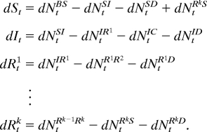 |
Fig. 1.

Diagrammatic representation of a model for cholera population dynamics. Each individual is in S (susceptible), I (infected), or one of the classes Rj (recovered). Compartments B, C, and D allow for birth, cholera mortality, and death from other causes, respectively. The arrows show rates, interpreted as described in the text.
The population size Pt is presumed known, interpolated from census data. Transmission is stochastic, driven by Gaussian white noise
 |
In Eq. 3, we ignore stochastic effects at a demographic scale (infinitesimal variance proportional to St). We model the remaining transitions deterministically
 |
Time is measured in months. Seasonality of transmission is modeled by log(βt) = Σk=05 bksk(t), where {sk(t)} is a periodic cubic B-spline basis (31) defined so that sk(t) has a maximum at t = 2k and normalized so that Σk=05 sk(t) = 1; ε is an environmental stochasticity parameter (resulting in infinitesimal variance proportional to St2); ω corresponds to a non-human reservoir of disease; βtIt/Pt is human-to-human transmission; 1/γ gives mean time to recovery; 1/r and 1/(kr2) are respectively the mean and variance of the immune period; 1/m is the life expectancy excluding cholera mortality, and mc is the mortality rate for infected individuals. The equation for dNtBS in Eq. 4 is based on cholera mortality being a negligible proportion of total mortality. The stochastic system was solved numerically using the Euler–Maruyama method (32) with time increments of 1/20 month. The data on observed mortality were modeled as yt ∼ 𝒩[Ct − Ct−1, τ2(Ct − Ct−1)2], where Ct = NtIC. In the terminology given above, the state process xt is a vector representing counts in each compartment.
Results
Testing the Method Using Simulated Data.
Here, we provide evidence that the MIF methodology successfully maximizes the likelihood. Likelihood maximization is a key tool not just for point estimation, via the maximum likelihood estimate (MLE), but also for profile likelihood calculation, parametric bootstrap confidence intervals, and likelihood ratio hypothesis tests (34).
We present MIF on a simulated data set (Fig. 2A), with parameter vector θ* given in Table 1, based on data analysis and/or scientifically plausible values. Visually, the simulations are comparable to the data in Fig. 2B. Table 1 also contains the resulting estimated parameter vector θ̂ from averaging four MIFs, together with the maximized likelihood. A preliminary indicator that MIF has successfully maximized the likelihood is that ℓ(θ̂) > ℓ(θ*). Further evidence that MIF is closely approximating the MLE comes from convergence plots and sliced likelihoods (described below), shown in Fig. 3. The SEs in Table 1 were calculated via the sliced likelihoods, as described below and elaborated in Supporting Text. Because inference on initial values is not of primary relevance here, we do not present standard errors for their estimates. Were they required, we would recommend profile likelihood methods for uncertainty estimates of initial values. There is no asymptotic justification of the quadratic approximation for initial value parameters, since the information in the data about such parameters is typically concentrated in a few early time points.
Fig. 2.

Data and simulation. (A) One realization of the model using the parameter values in Table 1. (B) Historic monthly cholera mortality data for Dhaka, Bangladesh. (C) Southern oscillation index (SOI), smoothed with local quadratic regression (33) using a bandwidth parameter (span) of 0.12.
Table 1.
Parameters used for the simulation in Fig. 2A together with estimated parameters and their SEs where applicable
| θ* | θ̂ | SE(θ̂) | |
|---|---|---|---|
| b0 | −0.58 | −0.50 | 0.13 |
| b1 | 4.73 | 4.66 | 0.15 |
| b2 | −5.76 | −5.58 | 0.42 |
| b3 | 2.37 | 2.30 | 0.14 |
| b4 | 1.69 | 1.77 | 0.08 |
| b5 | 2.56 | 2.47 | 0.09 |
| ω × 104 | 1.76 | 1.81 | 0.26 |
| τ | 0.25 | 0.26 | 0.01 |
| ε | 0.80 | 0.78 | 0.06 |
| 1/γ | 0.75 | ||
| mc | 0.046 | ||
| 1/m | 600 | ||
| 1/r | 120 | ||
| k | 3 | ||
| ℓ | −3,690.4 | −3,687.5 |
Log likelihoods, ℓ, evaluated with a Monte Carlo standard deviation of 0.1, are also shown.
Fig. 3.

Diagnostic plots. (A–C) Convergence plots for four MIFs, shown for three parameters. The dotted line shows θ*. The parabolic lines give the sliced likelihood through θ̂, with the axis scale at the top right. (D–F) Corresponding close-ups of the sliced likelihood. The dashed vertical line is at θ̂.
Applying the Method to Cholera Mortality Data.
We use the data in Fig. 2B and the model in Eqs. 3 and 4 to address two questions: the strength of the environmental reservoir effect, and the influence of ENSO on cholera dynamics. See refs. 19 and 20 for more extended analyses of these data. A full investigation of the likelihood function is challenging, due to multiple local maxima and poorly identified combinations of parameters. Here, these problems are reduced by treating two parameters (m and r) as known. A value k = 3 was chosen based on preliminary analysis. The remaining 15 parameters (the first eleven parameters in Table 1 and the initial values S0, I0, R01, R02, R03, constrained to sum to P0) were estimated. There is scope for future work by relaxing these assumptions.
For cholera, the difference between human-to-human transmission and transmission via the environment is not clear-cut. In the model, the environmental reservoir contributes a component to the force of infection which is independent of the number of infected individuals. Previous data analysis for cholera using a mechanistic model (20) was unable to include an environmental reservoir because it would have disrupted the log-linearity required by the methodology. Fig. 4 shows the profile likelihood of ω and resulting confidence interval, calculated using MIF. This translates to between 29 and 83 infections per million inhabitants per month from the environmental reservoir, because the model implies a mean susceptible fraction of 38%. At least in the context of this model, there is clear evidence of an environmental reservoir effect (likelihood ratio test, P < 0.001). Although our assumption that environmental transmission has no seasonality is less than fully reasonable, this mode of transmission is only expected to play a major role when cholera incidence is low, typically during and after the summer monsoon season (see Fig. 5). Human-to-human transmission, by contrast, predominates during cholera epidemics.
Fig. 4.

Profile likelihood for the environmental reservoir parameter. The larger of two MIF replications was plotted at each value of ω (circles), maximizing over the other parameters. Local quadratic regression (33, 35) with a bandwidth parameter (span) of 0.5 was used to estimate the profile likelihood (solid line). The dotted lines construct an approximate 99% confidence interval (ref. 34 and Supporting Text) of (75 × 10−6, 210 × 10−6).
Fig. 5.

Superimposed annual cycles of cholera mortality in Dhaka, 1891–1940.
Links between cholera incidence and ENSO have been identified (18, 19, 46). Such large-scale climatic phenomena may be the best hope for forecasting disease burden (36). We looked for a relationship between ENSO and the prediction residuals (defined below). Prediction residuals are robust to the exact form of the model: they depend only on the data and the predicted values, and all reasonable models should usually make similar predictions. The low-frequency component of the southern oscillation index (SOI), graphed in Fig. 2C, is a measure of ENSO available during the period 1891–1940 (19); low values of SOI correspond to El Niño events. Rodó et al. (19) showed that low SOI correlates with increased cholera cases during the period 1980–2001 but found only weak evidence of a link with cholera deaths during the 1893–1940 period. Simple correlation analysis of standardized residuals or mortality with SOI reveals no clear relationship. Breaking down by month, we find that SOI is strongly correlated with the standardized residuals for August and September (in each case, r = −0.36, P = 0.005), at which time cholera mortality historically began its seasonal increase following the monsoon (see Fig. 5). This result suggests a narrow window of opportunity within which ENSO can act. This is consistent with the mechanism conjectured by Rodó et al. (19) whereby the warmer surface temperatures associated with an El Niño event lead to increased human contact with the environmental reservoir and greater pathogen growth rates in the reservoir. Mortality itself did not correlate with SOI in August (r = −0.035, P = 0.41). Some weak evidence of negative correlation between SOI and mortality appeared in September (r = −0.22, P = 0.063). Earlier work (20), based on a discrete-time model and with no allowance for an environmental reservoir, failed to resolve this connection between ENSO and cholera mortality in the historical period: to find clear evidence of the external climatic forcing of the system, it is essential to use a model capable of capturing the intrinsic dynamics of disease transmission.
Discussion
Procedure 1 depends on the viability of solving the filtering problem, i.e., calculating θ̂t and Vt in Eq. 2. This is a strength of the methodology, in that the filtering problem has been extensively studied. Filtering does not require stationarity of the stochastic dynamical system, enabling covariates (such as Pt) to be included in a mechanistically plausible way. Missing observations and data collected at irregular time intervals also pose no obstacle for filtering methods. Filtering can be challenging, particularly in nonlinear systems with a high-dimensional state space (dx large). One example is data assimilation for atmospheric and oceanographic science, where observations (satellites, weather stations, etc.) are used to inform large spatio-temporal simulation models: approximate filtering methods developed for such situations (4) could be used to apply the methods of this paper.
The goal of maximum likelihood estimation for partially observed data is reminiscent of the expectation–maximization (EM) algorithm (37), and indeed Monte Carlo EM methods have been applied to nonlinear state space models (24). The Monte Carlo EM algorithm, and other standard Monte Carlo Markov Chain methods, cannot be used for inference on the environmental noise parameter ε for the model given above, because these methods rely upon different sample paths of the unobserved process xt having densities with respect to a common measure (38). Diffusion processes, such as the solution to the system of stochastic differential equations above, are mutually singular for different values of the infinitesimal variance. Modeling using diffusion processes (as in above) is by no means necessary for the application of Procedure 1, but continuous-time models for large discrete populations are well approximated by diffusion processes, so a method that can handle diffusion processes may be expected to be more reliable for large discrete populations.
Procedure 1 is well suited for maximizing numerically estimated likelihoods for complex models largely because it requires neither analytic derivatives, which may not be available, nor numerical derivatives, which may be unstable. The iterated filtering effectively produces estimates of the derivatives smoothed at each iteration over the scale at which the likelihood is currently being investigated. Although general stochastic optimization techniques do exist for maximizing functions measured with error (39), these methods are inefficient in terms of the number of function evaluations required (40). General stochastic optimization techniques have not to our knowledge been successfully applied to examples comparable to that presented here.
Each iteration of MIF requires similar computational effort to one evaluation of the likelihood function. The results in Fig. 3 demonstrate the ability of Procedure 1 to optimize a function of 13 variables using 50 function evaluations, with Monte Carlo measurement error and without knowledge of derivatives. This feat is only possible because Procedure 1 takes advantage of the state-space structure of the model; however, this structure is general enough to cover relevant dynamical models across a broad range of disciplines. The EM algorithm is similarly “only” an optimization trick, but in practice it has led to the consideration of models that would be otherwise intractable. The computational efficiency of Procedure 1 is essential for the model given above, where Monte Carlo function evaluations each take ≈15 min on a desktop computer.
Implementation of Procedure 1 using particle filtering conveniently requires little more than being able to simulate paths from the unobserved dynamical system. The new methodology is therefore readily adaptable to modifications of the model, allowing relatively rapid cycles of model development, model fitting, diagnostic analysis, and model improvement.
Theoretical Basis for MIF
Recall the notation above, and specifically the definitions in Eqs. 1 and 2.
Theorem 1.
Assuming conditions (R1–R3) below,
 |
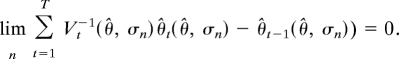
where ∇g is defined by [∇g]i = ∂g/∂θi and θ̂0 = θ. Furthermore, for a sequence σn → 0, define θ̂(n) recursively by
 |
where θ̂t(n) = θ̂t(θ̂(n), σn) and Vt,n = Vt(θ̂(n), σn). If there is a θ̂ with |θ̂(n) − θ̂|/σn2 → 0 then∇ log f(y1:T|θ = θ̂, σ = 0) = 0.
Theorem 1 asserts that (for sufficiently small σn), Procedure 1 iteratively updates the parameter estimate in the direction of increasing likelihood, with a fixed point at a local maximum of the likelihood. Step 2(ii) of Procedure 1 can be rewritten as θ̂(n+1) = V1,n{Σt=1T−1 (V t,n−1 − V t+1,n−1)θ̂t(n) + (V T,n−1)θ̂ T(n)}. This makes θ̂(n+1) a weighted average, in the sense that V1{Σt=1T−1 (V t−1 − V t+1−1) + V T−1)} = Idθ, where Idθ is the θ × dθ identity matrix. The weights are necessarily positive for sufficiently small σn (Supporting Text).
The exponentially decaying σn in step 2(i) of Procedure 1 is justified by empirical demonstration, provided by convergence plots (Fig. 3). Slower decay, σn2 = n−β with 0 < β < 1, can give sufficient conditions for a Monte Carlo implementation of Procedure 1 to converge successfully (Supporting Text). In our experience, exponential decay yields equivalent results, considerably more rapidly. Analogously, simulated annealing provides an example of a widely used stochastic search algorithm where a geometric “cooling schedule” is often more effective than slower, theoretically motivated schedules (41).
In the proof of Theorem 1, we define ft(ψ) = f(yt|y1:t−1, θt = ψ). The dependence on σ may be made explicit by writing ft(ψ) = ft(ψ, σ). We assume that y1:T, c and Σ are fixed: for example, the constant B in R1 may depend on y1:t. We use the Euclidean norm for vectors and the corresponding norm for matrices, i.e., |M| = sup|u|≤1 |u′Mu|, where u′ denotes the transpose of u. We assume the following regularity conditions.
R1. The Hessian matrix is bounded, i.e., there are constants B and σ0 such that, for all σ < σ0 and all θt ∈ ℝdθ, |∇2ft(θt, σ)| < B.
R2. E[|θt − θ̂t−1|2| y1:t−1] = O(σ2).
R3. E[|θt−θ̂t−1|3| y1:t−1] = o(σ2).
R1 is a global bound over θt ∈ ℝdθ, comparable to global bounds used to show the consistency and asymptotic normality of the MLE (42, 43). It can break down, for example, when the likelihood is unbounded. This problem can be avoided by reparameterizing to keep the model away from such singularities, as is common practice in mixture modeling (44). R2–R3 require that a new observation cannot often have a large amount of new information about θ. For example, they are satisfied if θ0:t, x1:t, and y1:t are jointly Gaussian. We conjecture that they are satisfied whenever the state space model is smoothly parametrized and the random walk θt does not have long tails.
Proof of Theorem 1.
Suppose inductively that |Vt| = O(σ2) and |θ̂t−1 − θ| = O(σ2). This holds for t = 1 by construction. Bayes' formula gives
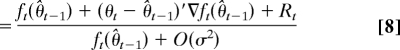 |
 |
The numerator in Eq. 8 comes from a Taylor series expansion of ft(θ̂t), and R1 implies |Rt| ≤ B|θt − θ̂t−1|2/2. The denominator then follows from applying this expansion to the integral in Eq. 7, invoking R2, and observing that Eq. 1 implies E[θt| y1:t−1] = θ̂t−1. We now calculate
 |
Eq. 11 follows from Eq. 10 using Eq. 9 and R3. Eq. 12 follows from Eq. 11 using the induction assumptions on θ̂t−1 and Vt; Eq. 12 then justifies this assumption for θ̂t. A similar argument gives
 |
where Eq. 14 follows from Eq. 13 via Eqs. 9 and 12 and the induction hypothesis on Vt. Eq. 14 in turn justifies this hypothesis. Summing Eq. 12 over t produces
 |
which leads to Eq. 5. To see the second part of the theorem, note that Eq. 6 and the requirement that |θ̂(n) − θ̂|/σn2 → 0 imply that
 |
Continuity then gives
 |
which, together with Eq. 5, yields the required result.
Heuristics, Diagnostics, and Confidence Intervals
Our main MIF diagnostic is to plot parameter estimates as a function of MIF iteration; we call this a convergence plot. Convergence is indicated when the estimates reach a single stable limit from various starting points. Convergence plots were also used for simulations with a known true parameter, to validate the methodology. The investigation of quantitative convergence measures might lead to more refined implementations of Procedure 1.
Heuristically, α can be thought of as a “cooling” parameter, analogous to that used in simulated annealing (39). If α is too small, the convergence will be “quenched” and fail to locate a maximum. If α is too large, the algorithm will fail to converge in a reasonable time interval. A value of α = 0.95 was used above.
Supposing that θi has a plausible range [θilo, θihi] based on prior knowledge, then each particle is capable of exploring this range in early iterations of MIF (unconditional on the data) provided is on the same scale as θihi − θilo. We use Σii1/2 = (θihi − θilo)/2 with Σij = 0 for i ≠ j.
Although the asymptotic arguments do not depend on the particular value of the dimensionless constant c, looking at convergence plots led us to take c2 = 20 above. Large values c2 ≈ 40 resulted in increased algorithmic instability, as occasional large decreases in the prediction variance Vt resulted in large weights in Procedure 1 step 2(ii). Small values c2 ≈ 10 were diagnosed to result in appreciably slower convergence. We found it useful, in choosing c, to check that [Vt]ii plotted against t was fairly stable. In principle, a different value of c could be used for each dimension of θ; for our example, a single choice of c was found to be adequate.
If the dimension of θ is even moderately large (say, dθ ≈ 10), it can be challenging to investigate the likelihood surface, to check that a good local maximum has been found, and to get an idea of the standard deviations and covariance of the estimators. A useful diagnostic, the “sliced likelihood” (Fig. 3B), plots ℓ(θ̂ + hδi) against θ̂i + h, where δi is a vector of zeros with a one in the ith position. If θ̂ is located at a local maximum of each sliced likelihood, then θ̂ is a local maximum of ℓ(θ), supposing ℓ(θ) is continuously differentiable. Computing sliced likelihoods requires moderate computational effort, linear in the dimension of θ. A local quadratic fit is made to the sliced log likelihood (as suggested by ref. 35), because ℓ(θ̂ + hδi) is calculated with a Monte Carlo error. Calculating the sliced likelihood involves evaluating log f(yt| y1:t−1, θ̂ + hδi), which can then be regressed against h to estimate (∂/∂θi) log f(yt| y1:t−1, θ̂). These partial derivatives may then be used to estimate the Fisher information (ref. 34 and Supporting Text) and corresponding SEs. Profile likelihoods (34) can be calculated by using MIF, but at considerably more computational expense than sliced likelihoods. SEs and profile likelihood confidence intervals, based on asymptotic properties of MLEs, are particularly useful when alternate ways to find standard errors, such as bootstrap simulation from the fitted model, are prohibitively expensive to compute. Our experience, consistent with previous advice (45), is that SEs based on estimating Fisher information provide a computationally frugal method to get a reasonable idea of the scale of uncertainty, but profile likelihoods and associated likelihood based confidence intervals are more appropriate for drawing careful inferences.
As in regression, residual analysis is a key diagnostic tool for state space models. The standardized prediction residuals are {ut(θ̂)} where θ̂ is the MLE and ut(θ) = [Var(yt| y1:t−1, θ)]−1/2 (yt − E[yt| y1:t−1, θ]). Other residuals may be defined for state space models (8), such as E|∫ t−1t dWs| y1:T, θ̂] for the model in Eqs. 3 and 4. Prediction residuals have the property that, if the model is correctly specified with true parameter vector θ*, {ut(θ*)} is an uncorrelated sequence. This has two useful consequences: it gives a direct diagnostic check of the model, i.e., {ut(θ̂)} should be approximately uncorrelated; it means that prediction residuals are an (approximately) prewhitened version of the observation process, which makes them particularly suitable for using correlation techniques to look for relationships with other variables (7), as demonstrated above. In addition, the prediction residuals are relatively easy to calculate using particle-filter techniques (Supporting Text).
Supplementary Material
Acknowledgments
We thank the editor and two anonymous referees for constructive suggestions, Mercedes Pascual and Menno Bouma for helpful discussions and Menno Bouma for the cholera data shown in Fig. 2B. This work was supported by National Science Foundation Grant 0430120.
Abbreviations
- ENSO
El Niño Southern Oscillation
- MIF
maximum likelihood via iterated filtering
- MLE
maximum likelihood estimate
- EM
expectation—maximization.
Footnotes
The authors declare no conflict of interest.
This article is a PNAS direct submission.
References
- 1.Anderson BD, Moore JB. Optimal Filtering. Engelwood Cliffs, NJ: Prentice-Hall; 1979. [Google Scholar]
- 2.Shephard N, Pitt MK. Biometrika. 1997;84:653–667. [Google Scholar]
- 3.Ionides EL, Fang KS, Isseroff RR, Oster GF. J Math Biol. 2004;48:23–37. doi: 10.1007/s00285-003-0220-z. [DOI] [PubMed] [Google Scholar]
- 4.Houtekamer PL, Mitchell HL. Mon Weather Rev. 2001;129:123–137. [Google Scholar]
- 5.Thomas L, Buckland ST, Newman KB, Harwood J. Aust NZ J Stat. 2005;47:19–34. [Google Scholar]
- 6.Brown EN, Frank LM, Tang D, Quirk MC, Wilson MA. J Neurosci. 1998;18:7411–7425. doi: 10.1523/JNEUROSCI.18-18-07411.1998. [DOI] [PMC free article] [PubMed] [Google Scholar]
- 7.Shumway RH, Stoffer DS. Time Series Analysis and Its Applications. New York: Springer; 2000. [Google Scholar]
- 8.Durbin J, Koopman SJ. Time Series Analysis by State Space Methods. Oxford: Oxford Univ Press; 2001. [Google Scholar]
- 9.Doucet A, de Freitas N, Gordon NJ, editors. Sequential Monte Carlo Methods in Practice. New York: Springer; 2001. [Google Scholar]
- 10.Kitagawa G. J Am Stat Assoc. 1998;93:1203–1215. [Google Scholar]
- 11.Gordon N, Salmond DJ, Smith AFM. IEE Proc F. 1993;140:107–113. [Google Scholar]
- 12.Liu JS. Monte Carlo Strategies in Scientific Computing. New York: Springer; 2001. [Google Scholar]
- 13.Arulampalam MS, Maskell S, Gordon N, Clapp T. IEEE Trans Sig Proc. 2002;50:174–188. [Google Scholar]
- 14.Sack DA, Sack RB, Nair GB, Siddique AK. Lancet. 2004;363:223–233. doi: 10.1016/s0140-6736(03)15328-7. [DOI] [PubMed] [Google Scholar]
- 15.Zo YG, Rivera ING, Russek-Cohen E, Islam MS, Siddique AK, Yunus M, Sack RB, Huq A, Colwell RR. Proc Natl Acad Sci USA. 2002;99:12409–12414. doi: 10.1073/pnas.192426499. [DOI] [PMC free article] [PubMed] [Google Scholar]
- 16.Huq A, West PA, Small EB, Huq MI, Colwell RR. Appl Environ Microbiol. 1984;48:420–424. doi: 10.1128/aem.48.2.420-424.1984. [DOI] [PMC free article] [PubMed] [Google Scholar]
- 17.Pascual M, Bouma MJ, Dobson AP. Microbes Infect. 2002;4:237–245. doi: 10.1016/s1286-4579(01)01533-7. [DOI] [PubMed] [Google Scholar]
- 18.Pascual M, Rodó X, Ellner SP, Colwell R, Bouma MJ. Science. 2000;289:1766–1769. doi: 10.1126/science.289.5485.1766. [DOI] [PubMed] [Google Scholar]
- 19.Rodó X, Pascual M, Fuchs G, Faruque ASG. Proc Natl Acad Sci USA. 2002;99:12901–12906. doi: 10.1073/pnas.182203999. [DOI] [PMC free article] [PubMed] [Google Scholar]
- 20.Koelle K, Pascual M. Am Nat. 2004;163:901–913. doi: 10.1086/420798. [DOI] [PubMed] [Google Scholar]
- 21.Finkenstädt BF, Grenfell BT. Appl Stat. 2000;49:187–205. [Google Scholar]
- 22.Liu J, West M. In: Sequential Monte Carlo Methods in Practice. Doucer A, de Freitas N, Gordon JJ, editors. New York: Springer; 2001. pp. 197–224. [Google Scholar]
- 23.Hürzeler M, Künsch HR. In: Sequential Monte Carlo Methods in Practice. Doucer A, de Freitas N, Gordon JJ, editors. New York: Springer; 2001. pp. 159–175. [Google Scholar]
- 24.Cappé O, Moulines E, Rydén T. Inference in Hidden Markov Models. New York: Springer; 2005. [Google Scholar]
- 25.Clark JS, Bjørnstad ON. Ecology. 2004;85:3140–3150. [Google Scholar]
- 26.Turchin P. Complex Population Dynamics: A Theoretical/Empirical Synthesis. Princeton: Princeton Univ Press; 2003. [Google Scholar]
- 27.Ellner SP, Seifu Y, Smith RH. Ecology. 2002;83:2256–2270. [Google Scholar]
- 28.Bjørnstad ON, Grenfell BT. Science. 2001;293:638–643. doi: 10.1126/science.1062226. [DOI] [PubMed] [Google Scholar]
- 29.Kermack WO, McKendrick AG. Proc R Soc London A; 1927. pp. 700–721. [Google Scholar]
- 30.Bartlett MS. Stochastic Population Models in Ecology and Epidemiology. New York: Wiley; 1960. [Google Scholar]
- 31.Powell MJD. Approximation Theory and Methods. Cambridge, UK: Cambridge Univ. Press; 1981. [Google Scholar]
- 32.Kloeden PE, Platen E. Numerical Solution of Stochastic Differential Equations. 3rd Ed. New York: Springer; 1999. [Google Scholar]
- 33.Cleveland WS, Grossel E, Shyu WM. In: Statistical Models in S. Chambers JM, Hastie TJ, editors. London: Chapman & Hall; 1993. pp. 309–376. [Google Scholar]
- 34.Barndorff-Nielsen OE, Cox DR. Inference and Asymptotics. London: Chapman & Hall; 1994. [Google Scholar]
- 35.Ionides EL. Stat Sin. 2005;15:1003–1014. [Google Scholar]
- 36.Thomson MC, Doblas-Reyes FJ, Mason SJ, Hagedorn SJ, Phindela T, Moore AP, Palmer TN. Nature. 2006;439:576–579. doi: 10.1038/nature04503. [DOI] [PubMed] [Google Scholar]
- 37.Dempster AP, Laird NM, Rubin DB. J R Stat Soc B. 1977;39:1–22. [Google Scholar]
- 38.Roberts GO, Stramer O. Biometrika. 2001;88:603–621. [Google Scholar]
- 39.Spall JC. Introduction to Stochastic Search and Optimization. Hoboken, NJ: Wiley; 2003. [Google Scholar]
- 40.Wu CFJ. J Am Stat Assoc. 1985;80:974–984. [Google Scholar]
- 41.Press W, Flannery B, Teukolsky S, Vetterling W. Numerical Recipes in C++ 2nd Ed. Cambridge, UK: Cambridge Univ Press; 2002. [Google Scholar]
- 42.Cramér H. Mathematical Methods of Statistics. Princeton: Princeton Univ Press; 1946. [Google Scholar]
- 43.Jensen JL, Petersen NV. Ann Stat. 1999;27:514–535. [Google Scholar]
- 44.McLachlan G, Peel D. Finite Mixture Models. New York: Wiley; 2000. [Google Scholar]
- 45.McCullagh P, Nelder JA. Generalized Linear Models. 2nd Ed. London: Chapman & Hall; 1989. [Google Scholar]
- 46.Bouma MJ, Pascual M. Hydrobiologia. 2001;460:147–156. [Google Scholar]
Associated Data
This section collects any data citations, data availability statements, or supplementary materials included in this article.