

Abstract
Resting-state functional magnetic resonance imaging (fMRI) has been used to study brain networks associated with both normal and pathological cognitive function. The objective of this work is to reliably compute resting state network (RSN) topography in single participants. We trained a supervised classifier (multi-layer perceptron; MLP) to associate blood oxygen level dependent (BOLD) correlation maps corresponding to pre-defined seeds with specific RSN identities. Hard classification of maps obtained from a priori seeds was highly reliable across new participants. Interestingly, continuous estimates of RSN membership retained substantial residual error. This result is consistent with the view that RSNs are hierarchically organized, and therefore not fully separable into spatially independent components. After training on a priori seed-based maps, we propagated voxel-wise correlation maps through the MLP to produce estimates of RSN membership throughout the brain. The MLP generated RSN topography estimates in individuals consistent with previous studies, even in brain regions not represented in the training data. This method could be used in future studies to relate RSN topography to other measures of functional brain organization (e.g., task-evoked responses, stimulation mapping, and deficits associated with lesions) in individuals. The multi-layer perceptron was directly compared to two alternative voxel classification procedures, specifically, dual regression and linear discriminant analysis; the perceptron generated more spatially specific RSN maps than either alternative.
Keywords: fMRI, Resting State Network, Multilayer Perceptron, Functional Connectivity, Supervised Classifier, Brain Mapping
1 Introduction
Biswal and colleagues first described resting state functional magnetic resonance imaging (fMRI) in 1995 (Biswal et al., 1995). The literature in this field has since been growing exponentially (Snyder and Raichle, 2012). Most of this work has been directed towards describing the statistical properties of intrinsic blood oxygenation level dependent (BOLD) signal fluctuations in health and disease (Biswal et al., 2010; Fox and Greicius, 2010; Pievani et al., 2011; Zhang and Raichle, 2010). Spontaneous BOLD activity recapitulates, in the topographies of its temporal covariance structure, task-based fMRI responses to a wide variety of behavioral paradigms (Smith et al., 2009). These topographies currently are known as resting state networks (RSNs) or, equivalently, intrinsic connectivity networks (ICNs). RSNs have now been mapped over virtually all of the cerebral cortex as well as many subcortical structures including the cerebellum (Buckner et al., 2011; Choi et al., 2012; Lee et al., 2012; Power et al., 2011; Yeo et al., 2011). Critically, although RSN topographies differ across individuals (Mennes et al., 2010; Mueller et al., 2013), previously reported results generally have been reported at the group level. Effectively capturing individual differences in RSN organization would enhance the study of how intrinsic activity accounts for individual differences in human behavior and cognition. Reliable RSN mapping in individuals has multiple applications, for example, in the study of the physiological basis of inter-individual differences in cognition, e.g., (Cole et al., 2012; Koyama et al., 2011). Similarly, improved RSN mapping in individuals could be useful in the study of how focal lesions, e.g., strokes, lead to performance deficits (Carter et al., 2010; Golestani et al., 2013; He et al., 2007); such studies are difficult at the group level because of lesion heterogeneity. Yet another application is to improve the delineation of “eloquent” cortex prior to neurosurgery, to potentially reduce iatrogenic deficits (Otten et al., 2012; Tie et al., 2013; Zhang et al., 2009). Pre-operative task-fMRI has been used for this purpose (Wurnig et al., 2013) but often fails because patients are unable to comply with task paradigms. Lastly, individual RSN mapping could enhance functional co-registration, i.e., using RSN features to refine anatomical registration (Conroy et al., 2013; Sabuncu et al., 2010).
Two analytic strategies, seed-based correlation mapping (Biswal et al., 2010) and spatial independent components analysis (sICA) (Beckmann, 2012), have so far dominated the field of resting state fMRI. RSNs obtained by sICA are theoretically unbiased by prior assumptions. However, ICA is not robust at the single subject level; results obtained by this technique invariably are reported at the group level. Seed-based correlation mapping uses priors if it is limited to only a few seeds. However, systematically defining many seeds over the entire brain (Wig et al., 2013) and analyzing the results using graph theoretic tools (Power et al., 2011) or inner product based clustering (Lee et al., 2012; Yeo et al., 2011) effectively achieves independence from priors. Both ICA and systematic seed-based correlation mapping exemplify unsupervised learning. Therefore, RSNs obtained by these methods may differ not only in topography (i.e., extent and shape), but also in topology (i.e., number of distinct nodes making up a single RSN), depending on the granularity of the recovered components within the modular hierarchy of RSNs (Meunier et al., 2010). To illustrate, the default mode network (DMN) is a constellation of regions including the posterior cingulateprecuneus cortex (PCC), midline prefrontal cortex, lateral parietal cortex, superior frontal cortex and posterior cerebellum. The DMN may be recovered in its entirety (Fox et al., 2005) using highly supervised methods. However, unsupervised strategies variably recover the DMN in fragments (Kahn et al., 2008; Smith et al., 2009), or combined with fragments of other networks (Doucet et al., 2011; Lee et al., 2012; Yeo et al., 2011). Such inconsistencies stem from the fact that unsupervised learning procedures are not constrained to a particular topological scale; therefore, some post-hoc classification strategy (e.g., template matching) must be used to establish RSN identity.
The present work is fundamentally different in that the objective is not to discover RSNs nor to study their functional relevance, but rather to map the topography of known RSNs in individuals. To this end, we trained a multi-layer perceptron (MLP) to estimate RSN memberships of brain loci on the basis of BOLD correlation maps. A perceptron is a feed-forward artificial neural network, originally modeled on the human visual system, trained to associate weighted sums of input features with pre-defined output classes (Rosenblatt, 1958). After training, the MLP decision boundaries are fixed; thus, subsequent results are guaranteed to represent the same entity (at the same topological scale) across individuals or populations. Perhaps the best-known application of perceptrons is to recognize (classify) handwritten digits (Lecun et al., 1989). This application has obvious utility in automatic routing of letters at the post office. To distinguish between supervised vs. unsupervised learning, consider discovering the characters used to represent numbers in the decimal system by analysis of a large sample of addressed letters. This is very different from training a perceptron to read (classify) known numerals, e.g., zip codes on addressed letters. Analogously, RSN discovery, using group sICA or any other unsupervised method, is very different from preparing a trained MLP to map known RSNs in new subjects.
In the above example, each character must represent one and only one numeral. However, we do not assume that every brain region belongs to a single RSN. We allow each locus in the brain to belong to any RSN to a variable degree. Accordingly, RSN membership estimation represents regression rather than classification. However, classification and regression are closely related mathematically. MLP outputs, which approximate posterior probabilities of class membership (Ruck et al., 1990), can be converted to hard classifications by identifying the output class of greatest magnitude. We report both continuous RSN estimates and hard classifications (“winner-take-all” maps). MLP performance was characterized by residual error for the former and receiver operating characteristic (ROC) analysis for the latter (Section 2.4.3).
Our methodology represents a solution to an engineering problem, namely, mapping RSNs in individuals. However, MLP training performance offers valuable information about the structure and separability of resting-state networks. Differential performance across RSNs may provide insight into their relative inter-subject variability and complexity. MLP performance also provides an objective measure of data quality that can be used to study the effects of varying acquisition and preprocessing methodologies. We demonstrate this concept by determining the quantity of BOLD data required to reliably compute RSN topography in individual subjects. Similarly, we empirically determine the optimal ROI size for generation of correlation map training data. As a final result, two alternative strategies for extending group-level RSN topographies to individuals (linear discriminant analysis and dual regression) are compared to the MLP. This comparison shows that the MLP provides superior RSN mapping specificity.
2 Methods
The Methods section is organized as follows: We first describe the fMRI datasets (section 2.1) and neuroimaging methods (2.2). We next describe the task-fMRI meta-analyses (2.3) used to isolate seed ROIs. These seeds were used to generate the MLP training data. MLP-specific methodology is divided into design (2.4) and application (2.5). The design phase (2.4) used correlation maps corresponding to seed ROIs with categorical RSN labels to train (2.4.2), evaluate (2.4.3), and optimize (2.4.4, 2.4.5) the MLP. Application of the trained perceptron to individuals generated voxel-wise estimates of RSN membership throughout the brain (2.5). MLP results then were compared to dual regression (DR) and linear discriminant analysis (LDA) (2.6).
2.1 Participants
Perceptron training, optimization and validation used data sets previously acquired at the Neuroimaging Laboratories (NIL) at the Washington University School of Medicine. A second, large validation data set was obtained from the Harvard-MGH Brain Genomics Superstruct Project (Yeo et al., 2011). All patients were young adults screened to exclude neurological impairment and psychotropic medications. Demographic information and acquisition parameters are given in Table 1.
Table 1.
Characteristics of the Training, Test and Validation datasets.
| Dataset | Training | Optimization | Validation 1 | Validation 2§ |
|---|---|---|---|---|
| Number of Subjects | 21 (7M + 14 F) | 17 (8M + 9F) | 10 (4M + 6F) | 692 (305M + 387F) |
| Age in years | 27.6 (23–35) | 23.1 (18–27) | 23.3 ± 3 (SD) | 21.4 ± 2.4 (SD) |
| Scanner | Allegra | Allegra | Allegra | Tim Trio |
| Acquisition voxel size | (4 mm)3 | (4 mm)3 | (4 mm)3 | (3 mm)3 |
| Flip angle | 90° | 90° | 90° | 85° |
| Repetition Time (sec) | 2.16 | 2.16 | 3.03* | 3.00 |
| Number of frames | 128 × 6 runs | 194 × 4 runs | 110 × 9 runs | 124 × 2 runs |
| Citation | (Lee et al., 2012) | (Fox and Raichle, 2007) | (Fox et al., 2005) | (Yeo et al., 2011) |
Validation data set 1 included a one second pause between frames to accommodate simultaneous electroencephalography (EEG) recording.
Validation data set 2 was acquired at Harvard-MGH by the Brain Genomics Superstruct Project.
2.2 Neuroimaging methods
2.2.1 MRI acquisition
Imaging was performed with a 3T Allegra (NIL) or Tim Trio (Harvard-MGH) scanner. Functional images were acquired using a BOLD contrast sensitive gradient echo echo-planar sequence [parameters listed in Table 1] during which participants were instructed to fixate on a visual cross-hair, remain still and not fall asleep. Anatomical imaging included one sagittal T1-weighted magnetization prepared rapid gradient echo (MP-RAGE) scan (T1W) and one T2-weighted scan (T2W).
2.2.2 fMRI preprocessing
Initial fMRI preprocessing followed conventional practice (Shulman et al., 2010). Briefly, this included compensation for slice-dependent time shifts, elimination of systematic odd-even slice intensity differences due to interleaved acquisition (Supplemental text section S2.2.2) and rigid body correction of head movement within and across runs. Atlas transformation was achieved by composition of affine transforms connecting the fMRI volumes with the T2W and T1W structural images. Head movement correction was included with the atlas transformation in a single resampling that generated volumetric timeseries in (3mm)3 atlas space. Additional preprocessing in preparation for correlation mapping included spatial smoothing (6 mm full width at half maximum (FWHM) Gaussian blur in each direction), voxel-wise removal of linear trends over each fMRI run and temporal low-pass filtering retaining frequencies below 0.1 Hz.
Spurious variance was reduced by regression of nuisance waveforms derived from head motion correction and timeseries extracted from regions (of “non-interest”) in white matter and CSF. Nuisance regressors included also the BOLD timeseries averaged over the brain (Fox et al., 2005), i.e., global signal regression (GSR). Thus, all computed correlations were effectively order 1 partial correlations controlling for variance shared across the brain. GSR has been criticized on the grounds that it artificially generates anticorrelations (Murphy et al., 2009). However, GSR fits well as a step preceding principal component analysis because it generates approximately zero-centered correlation distributions. As well, GSR enhances the spatial specificity in subcortical seed regions and reduces structured noise (Fox et al., 2009). The question of whether the left tail of a zero-centered correlation distribution (“anticorrelations”) is “false” (Damoiseaux and Greicius, 2009) or “tenuously interpretable” (Yeo et al., 2011) is irrelevant in the context of supervised learning.
Correlation maps were computed using standard seed-based procedures (Fox et al., 2009), i.e., by correlating the timeseries averaged over all voxels within the seed against all other voxels, excluding the first 5 (pre-magnetization steady-state) frames of each fMRI run. Seeds were 5 mm radius spheres initially and 10.5 mm radius spheres after optimization (see section 5.4.3). Additionally, we employed frame-censoring with a threshold of 0.5% root mean square frame-to-frame intensity change (Power et al., 2012; Smyser et al., 2010). Frame-censoring excluded 3.8 ± 1.1% of all magnetization steady-state frames from the correlation mapping computations. Correlation maps were Fisher z-transformed prior to further analyses.
2.2.3 Surface processing and gray matter definition
Cortical reconstruction and volume segmentation were performed using FreeSurfer (http://surfer.nmr.mgh.harvard.edu/) (Dale et al., 1999). Adequate segmentation was verified by inspection of the FreeSurfer-generated results in all datasets (Table 1). Cortical and subcortical gray matter regions were selected from the Training set segmentations, thresholded to obtain a conjunction of 30% of subjects, and then masked with an image of the average BOLD signal intensity across all subjects, thresholded at 80% of the mode value. This last step removed from consideration brain areas in which the BOLD signal is unreliable because of susceptibility artifacts. The resulting 30,981 voxels constituted the grey matter mask. For purposes of visualization, individual surfaces were deformed to a common space (Van Essen et al., 2012), producing consistent assignment of surface vertex indices with respect to gyral features across subjects. Final volumetric results for each subject were sampled onto surface vertices by cubic spline interpolation onto mid-thickness cortical surface coordinates.
2.3 Meta-analysis of task fMRI and generation of training data
ROIs representing distinct RSNs were isolated by meta-analysis of task-fMRI responses. We initially targeted 10 functional systems, each represented by a variable number of response foci derived from the literature (Table S1). The initial set of response foci was refined to ensure that all ROIs assigned to the same RSN generated maximally similar correlation maps and that ROIs assigned to different RSNs generated distinct correlation maps. These criteria yielded 169 ROIs representing 7 RSNs with high intra- and low inter-network correlation (Figures 1 and 2 and Table 2; see Supplemental text section 2.3 for algorithmic details). Thus, 3 of the original 10 networks were subsumed into the remaining networks. To these were added a nuisance category consisting of 6 ROIs in cerebrospinal fluid (CSF) spaces. The latter enabled the MLP to separate correlation patterns representing CSF vs. true RSNs. Computing correlation maps for each of the 175 seed regions in all 21 Training subjects produced 3,675 images used as training data. Each image in the Training set was masked to include only grey matter voxels, producing a 3,675 × 30,981 matrix. Similarly, 175 regions 17 subjects = 2,975 images, 175 regions · 10 subjects = 1,750 images and 175 regions · 692 subjects = 121,100 images, were computed in the Optimization, Validation 1, and Validation 2 data sets, respectively.
Figure 1.

Seed ROIs for generation of correlation map data. Seed ROIs resulting from a meta-analysis of task foci (see section 2.3) were defined in volume space. To visualize the surface variability of volume-defined regions, 5 mm radius spherical ROIs centered on stereotactically defined coordinates were projected onto surface reconstructions for each individual. Transparent regions indicate at least 20% surface overlap of ROIs across subjects. Opaque regions indicate at least 50% overlap. Figure S1 shows both hemispheres in slice format.
Figure 2.

Single-subject, voxel-wise estimation of RSNs using the trained MLP. A. Each locus produces one correlation map that ultimately results in N=7 MLP estimates of network membership at that locus. B. Each correlation map is masked to include only grey matter voxels and projected into principal component space. C and D. The masked image is passed through the neural network. See Appendix A and Figure A1 for details of MLP connections and training process. E. Output values converted to percentiles (uniform distribution over 0 to 1 interval) for surface displays. The 8th (nuisance component) MLP output is not illustrated.
Table 2.
Studies of functional co-activation used to generate seed ROIs.
| RSN | Expanded acronym | Citation | Task paradigm | Task contrast | Final seed ROIs |
|---|---|---|---|---|---|
| DAN | Dorsal Attention Network | (Shulman et al., 2009; Tosoni et al., 2012) | Rapid Serial Visual Presentation (RSVP) | Cue Type × Time | 28 |
| (Shulman et al., 2009; Tosoni et al., 2012) | Rapid Serial Visual Presentation (RSVP) | Cue Location × Cue Type × Time | |||
| (Astafiev et al., 2004; Corbetta et al., 2000; Kincade et al., 2005) | Posner Cueing Task | Time | |||
| VAN | Ventral Attention Network | (Astafiev et al., 2004; Corbetta et al., 2000; Kincade et al., 2005) | Posner Cueing Task | Invalid vs. Valid | 15 |
| (Dosenbach et al., 2007) | 10 different cognitive control tasks* | Graph theoretic analysis | |||
| SMN | Sensori-Motor Network | (Corbetta et al., 2000; Kincade et al., 2005) | Posner Cueing Task | Motor response | 39 |
| (Petacchi et al., 2005) | Various auditory stimuli | Stimulation vs. Control | |||
| VIS | Visual network | (Sylvester et al., 2008; Sylvester et al., 2007, 2009) | Visual Localizer | Discrete visual stimuli | 30 |
| FPC | Fronto-Parietal Control network | (Dosenbach et al., 2007) | 10 different cognitive control tasks* | Graph theoretic analysis | 12 |
| LAN | Language network | (Sestieri et al., 2011; Sestieri et al., 2010) | Perceptual vs. Episodic Memory Search Paradigm | Sentence reading | 13 |
| DMN | Default Mode Network | (Sestieri et al., 2011; Sestieri et al., 2010) | Perceptual vs. Episodic Memory Search Paradigm | Memory retrieval | 32 |
Regions reported by Dosenbach and colleagues (2007) were themselves the result of a meta-analysis.
2.4 MLP design
The core of a perceptron is an artificial neural network consisting of an input, hidden, and output layer, each consisting of nodes fully connecting to the next layer (all-to-all feed-forward). Training samples are passed into this feed-forward network and the output is compared to the a priori assigned RSN label. The error in this comparison is used to update the connection weights, between layers to increase the performance of the MLP (Rumelhart et al., 1986).
2.4.1. Principal components analysis (PCA) preprocessing
Expressing MLP inputs as eigenvector weights, in other words, preceding the MLP proper with a PCA layer, enabled dimensionality reduction without significant loss of information (Erkmen and Yɪldɪrɪm, 2008). PCA preprocessing allowed the use of fewer hidden layer nodes, reduced the size of the weight matrices and accelerated the training process by a factor of ~500. PCA was performed on the matrix of gray matter masked correlation images constituting the Training set (21 subjects · 175 seeds = 3,675 images, each image comprised of 30,981 gray matter voxels). Each correlation map then was represented as its projection along some number of PCs. The number of PCs, and correspondingly, the number of input nodes (Ni) was a hyper-parameter subject to optimization (see section 2.4.4). The number of PCs used to optimize global performance (minimize squared error summed over classes) was 2,500 (see Section 2.4.4).
2.4.2. MLP training
Training data, represented as vectors in PCA space, were presented to the MLP input layer. Each training example was associated with a desired output value determined by its a priori assigned RSN label. The MLP generated 8 (7 RSN and one CSF) output values for each training example. During training, these outputs were compared to the desired values (1 at the node corresponding to the a priori assigned label, 0 at other nodes). This comparison generated error signals used to update the connection weights. Algorithmic details are given in Appendix A, which includes a detailed schematic of the present MLP structure (Figure A1).
2.4.3. Quantitation of MLP performance
MLP error was defined as the difference between the MLP outputs and a priori assigned RSN labels (see above). Total RSN estimation performance was evaluated as root mean square (RMS) error aggregated over all output classes, across all training samples (participants × ROIs). Similar performance measures were computed for individual RSNs and individually for each participant.
Classification performance (in the winner-take-all sense) was quantified using receiver operator characteristic (ROC) analysis. ROC curves define the relation between the true positive fraction (TPF) vs. the false positive fraction (FPF) across a range of thresholds. An ROC curve was generated for each RSN. Thus, e.g., for the DAN, the TPF was the fraction of DAN training inputs above threshold at the DAN output node. Similarly, the FPF was the fraction of non-DAN inputs above threshold at the DAN output node. Thus, the area under the ROC curve (AUC) was used as a summary statistic representing classification performance for each RSN.
Training was paused at logarithmically spaced intervals during the training process and RMS error as well as AUC were calculated in the Optimization data set. This procedure produced training trajectories indicating the performance over-all and for each RSN throughout the training process.
2.4.4. Architecture selection
The number of PCs sampled (Ni), and the number of nodes in the hidden layer (Nh)constitute hyper-parameters subject to optimization. Overall RMS error was evaluated over a densely sampled Ni ∈ 5,6600 × Nh ∈ 4,5000 space. For each (Ni, Nh) coordinate, a MLP was trained until Optimization set error reached a minimum. This procedure was repeated (minimum of eight repetitions) for each (Ni, Nh) coordinate to identify the architecture with the least error. This procedure identified 2,500 PCs and 22 hidden layer nodes as the optimal architecture (see Supplemental section S2.4.4 and Figure S2). Similar systematic evaluation MLP performance as a function of ROI size identified 10.5mm as the optimum (Figure 10B).
Figure 10.

Examples of objective evaluation of methodology. A. Effect of total quantity of fMRI data on MLP performance. The plotted points (small triangles) represent total RMS error obtained with the fully trained MLP under three random sub-samplings of the Validation 1 dataset. RMS error (E) was fit to a 3-parameter rational function (red line). Asymptotic RMS error (~15.6%) was estimated from the function model. Note monotonically decreasing error with increasing data quantity. The large symbols report values for particular datasets: diamond: Training; circle: Optimization; triangle: Validation 1; square: Validation 2. The inset surface displays show the effect of available data quantity on WTA results. Note less RSN fragmentation with more data. B. Effect of Optimization ROI size on MLP performance. Each seed radius was evaluated with 5 replicates. Red line: locally linear scatterplot smoothing (LOESS, smoothing parameter of 0.5). Note clear minimum at approximately 10 mm radius.
2.4.5. Performance optimization by simulated annealing
After identifying the optimal architecture with least error in the Optimization data set, performance was iteratively optimized by simulated annealing (Kirkpatrick et al., 1983), countering the tendency of perceptrons to become trapped in local minima. Mimicking the random movement of atoms aligning in cooling metal, simulated annealing uses random perturbations of model parameters to find the global extremum in an objective function (Geman and Geman, 1984). Perturbations of steadily decreasing size (specified by a `cooling profile') are guaranteed to find a global minimum, although, in practice, the necessary cooling profile is prohibitively slow (Kirkpatrick, 1984). The cooling profile was designed to ensure that the sum of squares of the connection weights was unaltered by the simulated annealing perturbations and that most weights decreased while a few weights sporadically increased. Additional simulated annealing details are provided in Supplementary content (S2.4.5).
Error in the Optimization data was used as heuristic in the above-described iterative optimization procedure. Therefore, to avoid underestimating generalization error, final performance was estimated using a fully independent Validation datasets.
2.5 Application of method to individuals
To map RSNs in individual subjects, a correlation map was generated for every voxel in the brain and then propagated through the optimized perceptron. An overall schematic of this process is depicted in Figure 2.
2.5.1. Whole-brain analysis
Each of the 65,549 voxels in the brain generated a correlation map (Fig. 2A). Projecting correlation map values within the gray matter mask (30,981 voxels) into PCA space (see section 2.4.1) yielded 2,500 principal component coefficients (Fig. 2B). Thus, for each participant, the data presented to the MLP were contained in a 65,549 × 2,500 matrix (same 2,500 dimensional PCA space as used for MLP training). Each individual's data then were propagated through the perceptron (see section 2.4.2). The first layer (Fig. 2C) reduced the data to 22 features (65,549 × 22 matrix); the second layer (Fig. 2D) produced MLP outputs (65,549 × 8 matrix). These outputs were used to compute RMS error. RMS error served as the feedback signal during training and was also used to assess MLP performance. For display purposes, MLP output values were rank-order transformed to a uniform [0,1] distribution within each network. This transformation emphasizes topography rather than magnitude.
2.5.2. Group-level analyses
To visualize group-level results, RSN membership estimates were sampled onto the cortical mid-thickness surface for each participant. Averages were then computed across surface vertices. The standard deviation of MLP output values was also calculated vertex-wise to illustrate regions of high variability. To visualize group-level results in sub-cortical structures, MLP output values were averaged voxel-wise across participants. Group-average images were then re-sampled to 1mm cubic voxels and overlaid on a co-registered MNI152 atlas template.
2.6 Comparison of the MLP to linear discriminant analysis and dual regression
Linear discriminant analysis (LDA) is a classification algorithm that operates by projecting data onto vectors that maximize the ratio of between-class scatter to within-class scatter (Appendix B). PCA preprocessing is essential in LDA because the dimensionality of the input space (originally, tens of thousands of voxels) must be substantially less than the number of training examples (Belhumeur et al., 1997). By systematic exploration of the feasible PCA dimensionality range, it was determined that the lowest classification error in the Optimization set was obtained with 20 principal components. All present LDA results were obtained with this LDA design.
Dual regression (DR) is a technique commonly used subsequent to group ICA to extend spatial ICs discovered at the group level to individuals. Group ICA is a technique for discovering RSNs whereas the present work is about mapping known RSNs, not about RSN discovery (see Introduction). In fact, the present LAN (see section 2.3) typically is not obtained by group ICA, e.g., (Damoiseaux et al., 2006). Nevertheless, DR is algebraically well defined regardless of the origin of the group-level RSNs (Appendix B). Here, we used RSNs derived by meta-analysis of task-fMRI. Seed-based correlation maps were averaged across all participants and across all seed regions representing each class, generating 7 spatial RSN components and one nuisance component. Dual regression was then performed as described in Appendix B (cf. (Zuo et al., 2010)).
Voxel-wise RSN estimates were generated using each technique (MLP, DR, LDA) and converted to a percentile scale as described in section 2.5.1 for visualization. To quantitatively compare performance across methods, RSN estimates were computed for maps generated using the a priori ROIs. Seed-based covariance maps were used to evaluate DR performance (Eq. (B.5) in Appendix B); seed-based correlation maps were used to evaluate LDA and MLP performance (Eqs. (B.6) and (B.7)). These evaluations yielded RSN estimates for each seed for each participant for each method. From these values and the associated a priori RSN labels, ROC curves and AUC scores were computed for each network (see section 2.4.3).
3 Results
3.1 MLP training
3.1.1 Statistical properties of the training data
Temporal (Fig 3A) and spatial (Fig. 3B) correlation maps across seeds revealed distinct clustering corresponding to RSNs. Fig 3B exhibits two major clusters, one corresponding to the DAN, VAN, VIS and SMN networks, and the other corresponding to the FPC, LAN, and DMN networks. This dichotomy corresponds to the first principal component in Fig 3C. In the PC1 × PC2 plane (Fig. 3C), DAN (purple) and DMN (red) showed little overlap and appeared at opposite ends of the PC1 axis. VAN (magenta) and VIS (green) clusters were highly overlapping in this plane, but well separated in the PC3 × PC4 plane.
Figure 3.

Projection of RSNs into PCA space. A. Temporal correlation matrix: For each subject, the processed BOLD time-courses were averaged over each seed region. The resulting matrices were averaged across subjects. B. Spatial correlation matrix: For each subject, correlation maps were produced for every seed region. Matrices of spatial correlation between each seed's map were computed, and then averaged across subjects. C. Principal component analysis: PCA was performed on correlation maps, yielding the eigenvectors of the map-to-map spatial covariance matrix. Correlation maps for each seed in each subject were projected onto the PCA components, thus generating a locus in PCA space for each of the 3,675 training images. Color indicates the task analysis from which the region was derived.
3.1.2 Training Process
Figure 4 shows the training performance for the perceptron optimized for overall performance (2,500 input PCs, 22 hidden layer nodes). For every correlation map, each perceptron output node value represents an estimate of membership in a particular RSN.
Figure 4.
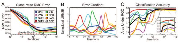
MLP Training trajectories as reflected in the Optimization dataset. A. Total RMS error as a function of iteration number. Error decreased monotonically for all networks until reaching a global minimum. The black line represents the total RMS error across all networks. The optimal early stopping point was defined as the global minimum of the total RMS error. B. Change in RMS error for each RSN (sign inverted derivatives with respect to iteration). The plotted values have been normalized by change in mean RMS error (black curve in A). Note sequential appearance of -ΔRMS error peaks and expanded iteration scale. C: ROC curves plotted in parallel with panel A. AUC values in the Training set asymptotically approached unity (not shown), whereas the Optimization data exhibited local maxima (inset). The black line represents the mean AUC across the 7 RSNs. Iterations index is shown on a logarithmic scale in all plots to emphasize early performance.
Perceptron outputs are initially centered at 0.5; as training progresses, within-class output values increase towards unity, while out-of-class output values decrease towards zero (see Fig. A3). RMS error across RSNs (Fig. 4A, black line) began near 0.5 and decreased monotonically until reaching peak performance (Fig. 4A, black arrow); training beyond this point resulted in over-fitting, i.e., decreasing performance (increasing RMS error) in the Optimization dataset despite increasing Training performance (see example in Figure A3).
For all networks, the AUC exhibited transient decrement in performance early in training (Fig. 4C). This feature corresponded to transient changes of slope in RMS error but did not produce concavity (local minima) in Fig. 4A. RMS error slopes indicated that class separation was achieved at varying numbers of iterations for different RSNs (Fig. 4B). The default mode network (red trace) achieved asymptotic performance earliest, and the language network (orange) latest. Asymptotic performance for the CSF class occurred much later than any true RSN.
3.2 MLP performance in the Validation datasets
3.2.1 Results in individuals
After completion of training, voxel-wise correlation maps were propagated through the MLP in the Validation datasets. Well-defined RSN topographies were obtained in all Validation dataset 1 participants (exemplars shown in Fig. 5). RSN topography summaries are displayed as winner-take-all maps (Fig. 5, lower panel). The worst Validation 1 AUC was 0.993 with an RMS error of 17.5%. In Validation dataset 2, the mean AUC was .977 with a SD of 0.0085; RMS error (mean ± SD) was 19.4% ± 1.73%. The systematically greater RMS error in Validation dataset 2 is accounted for by systematically less data (12 vs. 48 minutes; see Fig. 10A).
Figure 5.

RSN topographies in individual participants from Validation dataset 1. Voxel-wise MLP results are shown for 3 participants. These are the best, median, and worse performers as determined by RMS error. Voxelwise MLP output values have been converted to a percentile scale within each RSN and sampled onto each individual's cortical surface.
Figure 6 demonstrates the degree to which the MLP to captures individual variability. We first compared SMN topography to gyral morphology in 5 participants from Validation dataset 2. Participants were selected for display in Fig 6A as follows: The distribution of anterior-posterior (AP) positions the SMN (centroid over Talairach Z coordinate [+30,+45], left hemisphere, X coordinate < 15) was computed over all participants. One exemplar was randomly selected from each quintile. High SMN values conformed to the detailed morphological features of of the central sulcus in individuals (red arrows, Fig. 6A, Z = +53). High SMN values also tracked the AP position of the central sulcus (Fig. 6A, Z = +38). To obtain a quantitative measure of this tracking, the Y-coordinate of the SMN centroid and the fundus of the central sulcus were evaluated in Validation dataset 2 participants. The correlation between these positional measures was highly significant (r = 0.70, p < 10−15; Fig. 6B). This analysis was performed in [the first anonymized] 100 individuals because it required FreeSurfer segmentation of the cortical surface, which is computationally expensive.
Figure 6.

MLP SMN results obtained in Validation dataset 2 individuals. A: Five individuals were selected to represent the correspondence between SMN variability and anatomical variability in the central sulcus (see text for details). MLP SMN scores are displayed overlayed on individual MP-RAGE slices. The bright contour corresponds to the 90th percentile of voxel values. Note: high SMN scores track the shape of the central sulcus (red arrows). B: Correlation between the Talairach Y-coordinate of the centroid of MLP SMN (un-normalized) output values and the Y-coordinate centroid of the central sulcus fundus traced over the path indicated in the right inset figure. The SMN centroid was evaluated over the X–Y range indicated by the left inset figure.
3.2.2 Validation results at the group level
Figure 7 shows surface projections of RSN topography estimates averaged over 100 participants in Validation dataset 2. This figure addresses both the central tendency (top row) of each RSN, as well as inter-subject variability (middle row). As expected, average network topographies exhibited higher values (red) near locations of ROIs used to generate training maps (Fig. 1). More importantly, high RSN scores (in the top 25%) were consistently found in contiguous regions not used to generate training data. For example, a lateral temporal region was estimated as fronto-parietal control (Fig. 7, top row, FPC column), and high language network estimates were assigned to a dorsal pre-motor region (LAN column). These features are also present in the results in individuals (Fig. 5A). The significance of these observations with respect to external validity is discussed below (section 4.2).
Figure 7.

Surface-averaged MLP results. Top: Surface-based average over 100 participants from Validation dataset 2. Middle: Standard deviation of RSN values across subjects. Bottom: Winner-take-all maps depict surfaces with patches colored according to the network with the largest value.
Further evidence of external validity is shown in Figure 8, which includes all 692 participants in Validation dataset 2. For example, high SMN scores were obtained in thalamic voxels approximately corresponding to nucleus ventralis posterior and high VIS scores were obtained in posterior pulvinar (arrows), substantially in agreement with (Zhang et al., 2008). High VAN scores were obtained the dorso-medial nucleus, refining the parcellation in (Zhang et al., 2008), who identified this nucleus as functionally connected with “prefrontal” cortex. The posterior cerebellum (Crus I and II) and the cerebellar tonsils were assigned high DMN scores (Figure 7, Z = −30, Z= −47), in agreement with (Buckner et al., 2011). These results are noteworthy because neither cerebellar nor thalamic ROIs were used to generate training data. Further, no cerebellar voxels were within the grey matter mask, which means that the MLP correctly classified cerebellar voxels purely on the basis of cortical connectivity. High VAN and LAN RSN scores were asymmetrically obtained in the cerebellum (arrows, Z = −30), appropriately contralateral to asymmetric cerebral results (Z = +47).
Figure 8.

Volume-averaged MLP results 692 participants from Validation dataset 2, displayed in slices. WTA indicates the winner-take-all result (thresholded at 0.7 for the winning value). All seven networks were represented in the cerebellum despite absence of cerebellar seeds in the training data. Note left lateralized cerebral foci and right lateralized cerebellar foci for the language network (white arrows, LAN column); similarly, note right cerebral and left cerebellar foci for the ventral attention network (white arrows, VAN column).
3.3 Comparison of the MLP to alternative RSN estimation schemes
Dual regression (DR) and linear discriminant analysis (LDA) produced RSN topographies that were broadly similar to MLP results at the group level (Fig. 9A). However, DR and LDA topographies generally had greater spatial extent and more overlap across networks than the MLP-derived topographies. For example, the DAN network exhibited strong (greater than 90th percentile) values in dorsal SMN regions for both DR and LDA, but not for the MLP method. Similarly, VIS topography extended to SMN and DAN regions in DR results, less so in LDA results, and minimally in MLP results.
Figure 9.

Comparison of MLP to alternative methodologies. A. Selected group-average RSN topography estimates computed with dual regression (DR), linear discriminant analysis (LDA), and a multi-layer perceptron (MLP). B. RSN estimates evaluated over a priori seed ROIs. Topography estimates for each network (A) were averaged over voxels within each seed. The resulting scores were averaged over subjects and plotted for pairs of RSNs (e.g., SMN vs. VIS scores). Markers are colored based on the prior assignment of each seed. Line segments extend from the voxel-wise median score (50th percentile) to the center of mass of the ROI scores for the two RSNs defining the exhibited plane. Note that only the MLP successfully separates LAN seeds from DMN along the LAN axis. C. Inter-class correlation of RSN scores computed as the Pearson correlation coefficient between pairs of RSNs. Note that RSN scores are least correlated for the MLP, indicating more complete orthogonalization.
A cross-methodological comparison of classification performance in terms of AUC is given in Table 4. RSN scores were computed as described in section 2.6. These RSN scores were converted to hard classifications by identifying the group-derived map yielding the greatest score for each seed ROI. Linear Projection (LP), the simplest possible method, is included in Table 4 for comparison with the other methods (see Linear Projection in Appendix B). LP performance was evaluated using seed-based covariance maps (Eq. (B.1) in Appendix B). This is essentially nearest neighbor classification. That is, LP AUC is approximately equivalent to the probability that a map in, e.g., in PCA space is closest to the group average RSN template (represented by cluster centers in Figure 3C). Table 4 reports RMS error only for LDA and MLP results because the outputs generated by Linear Projection and DR are not confined to the interval [0,1] and cannot be directly compared to a priori labels.
Table 4.
RSN classification performance for alternative methodologies
| LP | DR | LDA | MLP | |||
|---|---|---|---|---|---|---|
| Network | AUC | AUC | AUC | RMSE | AUC | RMSE |
| DAN | 0.900 | 0.938 | 0.953 | 24.5% | 0.973 | 20.2% |
| VAN | 0.853 | 0.918 | 0.958 | 19.9% | 0.971 | 17.9% |
| SMN | 0.949 | 0.957 | 0.989 | 18.5% | 0.988 | 16.4% |
| VIS | 0.913 | 0.962 | 0.991 | 17.1% | 0.993 | 13.4% |
| FPC | 0.945 | 0.964 | 0.945 | 19.4% | 0.972 | 17.5% |
| LAN | 0.961 | 0.956 | 0.970 | 18.1% | 0.985 | 14.9% |
| DMN | 0.982 | 0.980 | 0.987 | 19.2% | 0.993 | 14.4% |
| Mean | 0.929 | 0.954 | 0.970 | 19.5% | 0.982 | 17.1% |
LP: Linear Projection; DR: dual regression; LDA: linear discriminant analysis; MLP: multi-layer perceptron. Data from the Optimization group (one correlation map per ROI per subject) were transformed by each method (Appendix B) to produce 7 RSN estimates per map. ROC analysis was performed to compute classification performance for each method. The differences between the RSN estimates and their ideal labels (d0 ∈ 0,1) were used to compute RMS error for LDA and MLP methods.
To illustrate the statistical covariance of RSN estimates, ROIs were plotted in planes defined by pairs of RSN scores (Figure 9B, top row). SMN ROIs (cyan cluster) achieved the highest score along the SMN axis in the SMN vs. VIS plane, and likewise for VIS ROIs. In plots for DR and LDA, DAN ROIs achieved relatively high scores in both dimensions (dark blue cluster in quadrant 1). This observation corresponds to the moderate spatial overlap between DAN, VIS, and SMN in DR results in Fig. 9A. SMN (cyan) and VIS (green) vectors extend from the median score to the center of mass of the ROI clusters. These vectors form an acute angle in the DR results, corresponding to generally correlated SMN vs. VIS estimates of network identity. LDA separates these vectors by a larger angle, which corresponds to less VIS-SMN spatial overlap. However, the DAN ROIs still achieve a high score on the VIS and SMN axes; the significant overlap of the DAN and SMN clusters corresponds to the spatial overlap of the DAN and SMN topographies in Fig. 9A.
In contrast, MLP showed greater within-network scores and lower across-network scores. For example, SMN and VIS ROIs achieved values near unity along their respective axes, while ROIs from other networks, notably DAN, achieved values closer to the median score. MLP output scores across anti-correlated networks also were closer to the median score. As might be expected, the contrast between MLP vs. either LDA or DR was especially marked in the case of difficult to separate RSNs, specifically, LAN vs. VAN and LAN vs. DMN.
Estimates of RSN identity were generally more correlated for DR and LDA methods than MLP. The Pearson correlation coefficient was computed (across all ROIs) for every pair of RSN classes, to generate inter-class correlation matrices in Figure 9C. The DR-derived inter-class correlation (Fig. 9C) retained more of the structure evident in Fig. 3B than the MLP-derived result. The magnitude of inter-class correlation was smaller for the MLP method than for either DR or LDA (p<0.05 and p<10−5, respectively, Mann-Whitney U-test), indicating that the MLP produced more orthogonal estimates of RSN membership than the other methods. Overall, classification performance was higher for the MLP (0.982 AUC) than for DR (0.954) and LDA (0.970).
4 Discussion
The perceptron in this study was trained to associate functional connectivity patterns (correlation maps) with 7 discrete RSNs. This number of RSNs corresponds to one particular scale of correlation structure of intrinsic human spontaneous fMRI activity (Lee et al., 2012; Yeo et al., 2011). After training, the perceptron recognized new correlation maps based on features of RSNs learned from the training data. Our results exploit the ability of the perceptron to operate outside the training data to generate voxel-wise estimates of network identity throughout the brain in individuals.
There are two primary measures of performance in this study. ROC analysis determines MLP performance as a classifier in the winner-take-all sense, i.e., categorical membership under the assumption that brain regions belong to a single RSN. RMS error indicates MLP performance as a regressor by measuring the deviation of a particular result from the ideal model of categorical membership. It is possible for the MLP to achieve perfect classification (AUC of unity) even when RMS error is far from zero. In fact, this is approximately what we found (Table 3). This result supports a view of the brain in which a given region may belong to multiple RSNs.
Table 3.
RSN classification (AUC) and estimation (RMS) performance.
| Training (N=21) | Optimization (N=17) | Validation 1 (N=10) | Validation 2 (N=692) | |||||
|---|---|---|---|---|---|---|---|---|
| Network | Accuracy (AUC) | Error (RMS) | Accuracy (AUC) | Error (RMS) | Accuracy (AUC) | Error (RMS) | Accuracy (AUC) | Error (RMS) |
| DAN | 0.992 | 15.7% | 0.973 | 20.8% | 0.973 | 21.1% | 0.966 | 23.1% |
| VAN | 0.991 | 14.9% | 0.971 | 19.6% | 0.979 | 17.7% | 0.962 | 21.0% |
| SMN | 0.998 | 15.3% | 0.988 | 20.0% | 0.994 | 17.5% | 0.983 | 23.4% |
| VIS | 0.998 | 11.1% | 0.993 | 14.9% | 0.998 | 12.5% | 0.993 | 16.5% |
| FPC | 0.988 | 12.7% | 0.972 | 17.1% | 0.989 | 14.8% | 0.971 | 17.7% |
| LAN | 0.993 | 13.5% | 0.985 | 16.0% | 0.991 | 14.5% | 0.979 | 17.7% |
| DMN | 0.997 | 13.9% | 0.993 | 19.7% | 0.991 | 17.5% | 0.986 | 20.3% |
| Mean | 0.994 | 13.6% | 0.982 | 17.8% | 0.988 | 16.2% | 0.977 | 19.5% |
These values reflect MLP training with 10.5 mm radius seeds (see Figure 10) and optimization with simulated annealing.
4.1 Inter-individual variability of MLP outputs
The present results (Figures 5–7) exhibit a high degree of face validity with respect to the training data and previously reported RSN results. Thus, for example, components of the DMN used as seeds to generate the training data were classified as DMN in all participants. This was true not only for easily classified networks (e.g., the DMN) but also for networks (e.g., VAN and LAN) that are inconsistently found by unsupervised procedures. The results shown in Figure 5 illustrate that the perceptron reliably classified RSNs in each individual in the Validation 1 group (0.984 worst case AUC), even in cases in which the RMS error was relatively high (> 0.175).
Analysis of voxelwise RSN membership estimates across a large cohort (100 subjects from Validation dataset 2) revealed RSN-specific zones of high as well as low inter-individual variability (Fig. 7, middle row). Voxels with high RSN scores generally showed the least inter-subject variability. Such regions, e.g., the posterior parietal component of the DMN (Fig. 7, right column), were surrounded by zones of high variability (e.g., a ring around the angular gyrus). The pre-and post-central gyri consistently showed high SMN RSN scores but were bordered by regions of high inter-subject SMN variability. Interestingly, inter-subject variability was low also in areas with RSN scores near 0, particularly in areas typically anticorrelated with other networks (e.g., low DAN variance in the angular gyrus, a component of the DMN; low DMN variance in MT+, a component of the DAN) (Fox et al., 2006).
At least four factors potentially contribute to observed inter-subject MLP output variability: (i) limited or compromised fMRI data; (ii) limitations intrinsic to the MLP; (iii) differences in RSN topography attributable to anatomic variability; (iv) true differences in RSN topography independent of variable gyral anatomy. We consider each of the possibilities in turn.
(i) The fMRI data used in the present work were obtained in healthy, cooperative young adults. Hence, the fraction of frames excluded because of head motion (Power et al., 2012) was low (about 4%). The total quantity of fMRI data acquired in each individual was generous by current standards (Van Dijk et al., 2010). However, fMRI data quantity clearly affects MLP performance (see section 4.5.2 below and Figure 10A). Current results suggest that more data generally improves MLP performance. The requirements for fMRI data quality and quantity for acceptable MLP performance in clinical applications remains to be determined. (ii) High variability in RSN boundary regions (e.g., Fig. 7, DMN, middle row) may reflect uncertainty attributable to multiple RSN membership, i.e., voxels with high “participation coefficients” (Guimera and Amaral, 2005; Power et al., 2011). Voxels with multiple RSN membership may be more difficult to classify because the training data included only maps derived from seeds assigned to single networks.
(iii) Figure 6 indicates that the MLP captures a substantial portion of anatomic variability. However, some part of MLP mapping imprecision may be explained by uncorrected anatomical variability. To investigate this possibility, we compared the overall RSN standard deviation map (Fig. S3A) to sulcal depth variability (Fig. S3B) and found a weak spatial correlation (r = 0.2). By inspection, these maps were concordant only at a broad spatial scale: both showed low variability in primary motor/auditory/insular cortices and high variability elsewhere. Little correspondence was evident at finer scales (note lack of annular patterns in Fig. S3B). The degree to which anatomical variability contributes to spurious variance in RSN topography estimates may be addressed by measuring the degree to which non-linear or surface-based registration decreases inter-subject variance and increases overall MLP performance (higher AUC, lower RMS error).
(iv) On the other hand, inter-individual differences may reflect “true” individual variability in RSN topography independent of gyral anatomy (Mueller et al., 2013). Previous work has demonstrated that inter-individual differences in task-evoked activity correspond to “transition zones” in resting state networks (e.g., the boundary between parietal DMN and DAN regions) (Mennes et al., 2010). These same regions appear in our inter-subject variance maps for both DMN and DAN (Fig. 7). We also note that areas of high RSN score variability (pre-frontal, parietal, lateral temporal) broadly correspond to regions exhibiting the greatest expansion over the course of human development and evolution (Hill et al., 2010). This correspondence may be coincidental, but it is consistent with the hypothesis that later developing or evolutionarily more recent areas of the brain tend to be more variable across individuals.
In summary, there are many potential contributions to observed RSN topographic variability. Because we did not use non-linear volume registration in this work, Fig. 6 retains individual differences in gyral anatomy. By inspection, the MLP was able to track these differences. Thus, it is reasonable to expect that the MLP will find “true” differences in RSN topography not attributable to variable gyral anatomy. Future studies are needed to compare MLP-derived topographies with, e.g., task-evoked responses, after correcting for anatomical variability.
4.2 External Validity and Generalizability
Two distinct types of external validity, that is, correct classification outside the Training set (areas covered by the seed ROIs), are evident in our results. First, high overall MLP performance was achieved for a priori seed-based correlation maps in the Optimization (98.2% AUC) and Validation 1 datasets (98.8% AUC). Performance was reliable in all participants (97.1% worst-case AUC), which is critical in clinical applications. Second, and perhaps of greater scientific interest, the RSN estimates in areas not covered by seed regions were strongly concordant with previously reported task-based and resting-state fMRI results. For example, while no temporal FPC seed ROI was included in the training set, a posterior temporal gyrus locus was classified as FPC (Lee et al., 2012; Power et al., 2011; Yeo et al., 2011) at the group level (Fig. 7, FPC column). Similarly, the MLP also identified the parahippocampal gyrus as DMN (Kahn et al., 2008).
The MLP identified as LAN components of dorsal and ventral streams previously associated with cortical speech processing (Hickok and Poeppel, 2004) see also (Binder et al., 2011). Whereas the ventral components were bilateral, the dorsal components were left lateralized (Fig. 8, white arrow, LAN column) (Hickok and Poeppel, 2007). This finding represents a strong demonstration of external validity, as the left dorsal region was not included in the Training set. The right inferior cerebellum was first associated with language function by PET studies of semantic association tasks (Petersen et al., 1988). Identification of this region here as part of the LAN network (Fig. 8, WTA, Z = −30 and −47) is doubly significant: First, no cerebellar seeds were used to generate training data and cerebellar voxels were excluded from the gray matter mask; hence, these voxels were not seen by the MLP. Second, lateralized cerebellar RSN components typically are not found by unsupervised seed-based correlation mapping (Buckner et al., 2011).
These findings highlight the capabilities of supervised learning applied to the problem of identifying RSNs in individuals. The cortical representation of language (primarily Broca's and Wernicke's areas) has been extensively studied using task-based fMRI (Binder et al., 2011) and correlation mapping with a priori selected ROIs (Briganti et al., 2012; Hampson et al., 2006; Pravata et al., 2011; Tomasi and Volkow, 2012). However, the language network, as presently defined, typically is not recovered as such by unsupervised methods, e.g., (Power et al., 2011; Yeo et al., 2011). Rather, components of the LAN are generally found only at fine-scale RSN descriptions. Thus, an RSN including Broca's and Wernicke's areas appears as the 11th of 23 components in (Doucet et al., 2011); these same areas were identified as VAN by Power and colleagues (2011) and DMN by Yeo and colleagues (2011). Lee et al., (2012), found a component consistent with the presently defined LAN at a hierarchical level of 11 (but not 7) clusters. Thus, the present work demonstrates the potential of supervised learning to find networks that are subtle features of the BOLD correlation structure. These may be minor sub-components within hierarchically organized RSNs or functional entities of high scientific interest or clinical value that do not fit within a hierarchical organization, i.e., extend over multiple levels or across multiple branches.
Because the MLP is a universal function approximator, it is subject to over-fitting. Over-fitting refers to learning features that are particular to the training set but that do not generalize to other sets. To minimize over-fitting, we halt training when Optimization dataset error reaches a minimum (Figure 4A). However, because early stopping is implemented throughout optimization by simulated annealing, over-fitting may still occur with respect to the Optimization dataset. Therefore, we demonstrate the performance of the fully trained MLP in two Validation datasets (Figs. 5–8).
4.3 Comparison of the MLP to dual regression (DR) and linear discriminant analysis (LDA)
The MLP, DR, and LDA all represent different strategies for extending RSN mapping results obtained at the group level to individuals. The MLP showed better spatial specificity of RSN estimates than either DR or LDA (Fig. 9A) and produced more orthogonal estimates of RSN identity in a priori ROIs (Fig. 9B). These comparative results indicate greater statistical independence of RSN estimates obtained by the MLP. However, perfect separation of classes was not achieved by any method, as indicated by residual correlation of RSN estimates (non-zero off-diagonal elements in Fig. 9C). This residual was greatest in the least separable RSNs (compare Figs. 9C and 2B).
Performance differences across the three methods can be related to their underlying algebraic structures, which reveal interesting commonalities as well as differences (Appendix B). All three methods operate by transforming individual voxel-wise covariance or correlation matrices into 7 dimensional RSN membership estimates at each voxel. However, the methods differ in the strategies used to achieve separation of RSN estimates. LDA requires considerable dimensionality reduction by PCA preprocessing. The optimal number of PCs was found to be 20, but this accounted for only 70% of the variance. In contrast, the MLP does not strictly require PCA preprocessing although this step greatly reduces the computational load without sacrificing information. In fact, the MLP performance optimum was obtained with 2,500 PCs (Figure S2), which included 99.97% of the variance. DR, as conventionally implemented (Zuo et al., 2010), does not involve PCA preprocessing or training.
Both LDA and MLP optimize separation of classes using thousands of labeled training samples, which captures variability across brain regions and individuals. Therefore, the superior performance of the MLP is not simply attributable to a large number of training samples. Rather, high-dimensional non-linear classification boundaries allow the MLP to extract arbitrary features from a large (2,500 PCs) input space. Future work will compare the MLP to LDA and DR in patients with focal lesions, i.e., stroke or brain tumors. At issue is performance under circumstances in which RSNs exhibit altered topography.
4.4 Dynamics of perceptron training reflect hierarchical brain organization
Several studies have demonstrated that resting state networks are hierarchically organized (Boly et al., 2012; Cordes et al., 2002; Doucet et al., 2011; Lee et al., 2012; Marrelec et al., 2008). Here, the hierarchical scale of an RSN is reflected in training performance trajectories (Fig. 4B): the DMN was the first to be separated from other RSNs. The DMN arguably is the most robust feature in the correlation structure of intrinsic brain activity. Its topography is very similar across RSN mapping strategies, specifically, spatial ICA (Beckmann et al., 2005) and seed-based correlation mapping (Yeo et al., 2011). Here, the DMN and regions anti-correlated with the DMN (Fox et al., 2005) were well separated along the first principal component of the training data (Figure 3)1.
After the DMN, the sensorimotor and visual networks were next to achieve separation (Fig. 4B). These networks are often seen at the next level down in the RSN hierarchy as offshoots of the anti-DMN (Lee et al., 2012) or `extrinsic system' (Doucet et al., 2011). The DAN achieved only a small peak in error descent compared to other `extrinsic' networks, although this occurred in close proximity to SMN and VIS. In contrast, the LAN and VAN were last to achieve separation. This corresponds to the observation that LAN and VAN systems are typically found by analyses extending to lower levels of the RSN hierarchy (Lee et al., 2012; Power et al., 2011).
4.5 MLP performance applied to the evaluation of fMRI methodology
4.5.1 Objective assessment of image quality
Modern imaging theory defines image quality as the capacity to enable an observer to perform a specific task (Barrett et al., 1998; Kupinski et al., 2003). Here, the observer is a multi-layer perceptron and the task is to assign RSN values (or labels) to each voxel. Performance is evaluated in terms of mean squared error and ROC analysis. It follows that MLP performance can be used to evaluate image quality across a wide range of variables, e.g., scanners, and acquisition parameters (repetition time, run length, resolution), preprocessing strategies (nuisance regression, filtering, spatial smoothing) and data representations (surface or volume based). We demonstrate this principle by systematically evaluating MLP performance in relation to quantity of fMRI data and seed ROI size.
4.5.2 Quantity of fMRI data
The relation between total quantity of fMRI data and MLP performance is shown in Figure 10A. The plotted points represent three random resamplings of all data in the Validation 1 dataset. RMS error as a function of data quantity was well fit (r2=0.994) by a three-parameter empirically derived rational function. The parameterized function implies that output RMS error monotonically decreases with increasing total fMRI data length but ultimately asymptotes at ~15.6%. The biological significance of this asymptote is discussed below (Section 4.6).
4.5.3. Optimal seed ROI size
The relationship between seed ROI radius and RMS error was explored using the optimal MLP architecture (2,500 PCs, 22 hidden nodes) determined with 5 mm radius seeds. All seeds were masked to include only gray matter voxels. The results of systematically varying seed ROI size are shown in Figure 10B. A clear minimum in RMS error was obtained with seeds of approximately 10.5 mm radius. Voxel-wise RSN topographies were qualitatively similar across ROI sizes, but larger seeds generated less noisy RSNs with more pronounced peaks. This result is unexpected, as it deviates from the current standard practice of using approximately 6 mm radius seeds (e.g., (Marrelec and Fransson, 2011)). There are several possible explanations for this result. Large seeds may best match the characteristic dimensions of RSNs in the 7-network level description of the brain. Alternatively, large seeds may compensate for mis-registration in affinecoregistered, volume-preprocessed data. We anticipate that smaller seeds will be optimal when estimating RSN membership of surface-coregistered, geodesically smoothed data. Hence, the results shown in Figure 10B should not be interpreted as unambiguously indicating that 10.5 mm radius seeds are optimal for correlation mapping in general. Rather, the large optimal radius (10.5 mm) indicates that averaging over more voxels outweighs loss of spatial specificity in this paradigm. Alternatively, the resultant increase in blurring may have corrupted the training data, which can lead to a more robust classifier (Dunmur and Wallace, 1993).
4.6 Limitations
The present MLP results were obtained using a particular set of RSNs selected for their scientific and clinical value in the context of ongoing research. A different training set including other RSNs might be optimal in other circumstances. MLP performance may be expected to vary with the number and separability of RSNs being classified as well as the total duration (Fig. 10A) and quality of acquired resting state fMRI data.
As discussed above (section 4.1), inter-individual differences in computed RSN topographies may reflect multiple factors. Cross-gyral contamination due to the relatively large voxels used in this study (3–4 mm acquisition, 3 mm post-processing analyses) may limit the precision of RSN estimation in our dataset (see (Yeo et al., 2011) for a discussion of this issue). Of greater theoretical importance is that we cannot distinguish between correctly identified geodesic (parallel to the cortical surface) shifts of RSN topography versus morphological differences in gyral/sulcal anatomy. Potential strategies for validating MLP-derived results individuals include comparison with measures of structural connectivity (Damoiseaux and Greicius, 2009) and invasive electrophysiologic recording (He et al., 2008).
As shown in Figure 3B as well as in prior work (Boly et al., 2012; Doucet et al., 2011; Lee et al., 2012; Marrelec et al., 2008), RSNs are hierarchically organized. Thus, a major dichotomy separates the `extrinsic' (DAN, VAN, VIS, SMN) from `intrinsic' networks (FPC, LAN, DMN). At the next level of granularity, RSN blocks are distinguishable within the major dichotomy. However, the cognitive domains corresponding to these RSNs (e.g., `motor', `language', `attention', etc.) are not conventionally regarded as hierarchically organized. Our training labels are categorical because they were generated from task-fMRI responses corresponding to conventionally understood cognitive domains (Table 2). Thus, this work is fundamentally limited in that we impose a `flat' conceptualization of brain function onto an intrinsically hierarchical system. This is reflected in the fact that ROIs are almost perfectly classified (by the AUC measure) in all datasets, yet RMS error always remains substantial (15%–20%) (Table 3, Fig. 10A). The existence of this residual may indicate that resting-state brain networks are inherently non-separable in the sense of classification. Indeed, this is consistent with the notion of “near decomposability” of hierarchical systems formed by multiple, sparsely inter-connected modules (Simon, 1995); this concept has been extended to brain networks (Meunier et al., 2010).
Another potential limitation is that all present analyses assume temporal stationarity, as do the overwhelming majority of extant papers on intrinsic BOLD activity. However, a growing literature (Chang and Glover, 2011; Kiviniemi et al 2011; Hutchinson et al 2012; Allen et al 2012) indicates that resting state correlation patterns fluctuate on a time scale of minutes. Our analysis of the effect on classifier performance of varying the total quantity of fMRI data (Fig. 10A) utilized contiguous epochs to the extent possible given fMRI runs of duration ~5 minutes. Less data reliably yielded worse performance. This result may be attributable either to sampling error (i.e., limited signal to noise ratio) or true temporal non-stationarities or both. Similarly, the performance floor may reflect non-stationarities. Disambiguating these possibilities would require much longer contiguous acquisitions.
4.7 Summary
The MLP estimates RSN membership at the voxel level via computed correlation maps. After training, it reliably identifies RSN topographies in individuals. RSN estimation is rapid (2 minutes using Matlab running on Intel i7 processors) and automated, hence suitable for deployment in clinical environments. After training, operation is independent of any particular seed. Therefore, the trained MLP is expected to be robust to anatomical shifts and distortions, for example, owing to enlarged ventricles and mass effects or even loss of neural tissue (e.g., stroke).
In this work, the MLP was trained to operate in 3D image space for compatibility with clinical imaging formats. However, the MLP concept can be readily adapted to operate on correlation maps represented on the cortical surface. Similarly, an MLP can be trained to ignore anatomical abnormalities (e.g., brain tumors) by altering the domain of the training set, i.e., excluding tumor voxels. This possibility will be explored in future work.
Supplementary Material
Highlights
A multilayer perceptron can accurately classify correlation maps into canonical RSNs.
Operating voxel-wise, the classifier produces full-brain topographies of RSNs.
RSN topographies at the group level are highly concordant with prior studies.
Classifier performance can be used to objectively optimize BOLD methodology.
Whole-brain classification is rapid and automated, thus suitable for clinical use.
Acknowledgments
This work was supported by the National Institute of Mental Health (RO1s MH096482-01 to Drs. Corbetta and Leuthardt), the National Cancer Institute (R21CA159470-02 to Dr. Leuthardt), Child and Health Development (R01 HD061117-05A2 to Dr. Corbetta), the National Institute of Stroke and Neurologic Disorders (P30 NS048056 to Dr. Snyder), National Institute of Health P50NS006833 to Dr. Snyder. This research was also supported by a research training grant from the University of Chieti, “G. d'Annunzio,” Italy (for Dr. Baldassarre) and the McDonnell Center Higher Brain Function. Validation dataset 2 was obtained from The Brain Genomics Superstruct Project, funded by the Simons Foundation Autism Research Initiative. We thank Matt Glasser for help with surface reconstruction and coregistration.
Appendix A
The input to the MLP algorithm consists of correlation maps projected onto eigenvectors computed by PCA preprocessing of the training data (see main text section 2.4.1). Each input's loadings onto the i-th eigenvector, yi, is formally defined as the output value of the i-th input layer node. This corresponds to the first layer in Fig. A1.
The total input to a hidden or output layer node, vh or vo, respectively, is computed as the sum of all output values from the previous layer weighted by feed-forward connections:
| (A.1) |
where i, h, and o index input, hidden, and output nodes; yh indicates the output value received from hidden layer node h; whi indicates the connection weights from input node i to hidden layer node h, and similarly for hidden to output layer connections woh. In this work, connection weights were initialized by sampling values from a uniform distribution over the interval [−0.01, 0.01].
Total inputs to each node are transformed into output values by layer-specific activation functions, φh and φo, which are the hyperbolic tangent and logistic curves, respectively:
| (A.2) |
where b = 0.1. The hidden node index, h, ranges from 1 to 22. The output node index, O, ranges from 1 to 8.
The overall transfer function of the perceptron is given in Eq. (A.3). This formula represents the propagation of inputs through the MLP (Figure A1):
| (A.3) |
After propagation of the input data, the output value for each node, yo, is compared to the a priori RSN output labels, do ∈ 0,1 , to find the error eo = do - yo. The total squared error, summed across all output nodes and all training samples, is given by E. The local gradient of the total error at output node o is computed as:
| (A.4) |
where the prime notation indicates the first derivative of φo (see application of chain rule in Eq. 4 in (Rumelhart et al., 1986)). Note that the derivative of the input, vo, with respect to the weights, woh, in Eq. (A.1) is simply the output from the previous layer, yh. The chain rule can therefore be used to calculate how total error changes with respect to the weights, i.e., . This gradient can thus be used to adjust the connection weights:
| (A.5) |
where η is the instantaneous learning rate (see Eq. (A.9) below and Fig. A2) and k is the iteration index. The weights to the hidden layer from the input layer are similarly adjusted:
| (A.6) |
However, the local gradient of the error at hidden node h, δh, must be computed indirectly by back-propagation of the local gradient of error at the output layer, weighted by the connections between the hidden and output layers:
| (A.7) |
The present results were obtained using an empirically determined learning rate parameter schedule, η k, which depended on the iteration index, k. The range of η values yielding stable learning was determined, where instability was defined as divergence or oscillation of classifier weights or output values. The learning rate schedule adaptively increased as a sigmoid in log iteration index (Fig. A2):
| (A.8) |
Thus, A = 5·10−4 = η(0) was the initial learning rate and K = 2·10−3 = η ∞ the maximal rate; B=−3; M = 2.5. The presently reported η values provided stable learning with double precision computations for the final architecture described in this work. Architectures with larger weight matrices required smaller values of η.
Appendix B - Algebraic comparison of methods
This appendix describes the algebraic relationship between dual regression (DR), linear discriminant analysis (LDA), and the multi-layer perceptron (MLP). We demonstrate that all three methods act on the second-order statistics over voxel pairs (covariance for DR and correlation and for LDA and MLP). Each method computes subject-level descriptions of group-defined spatial components.
B.1 Defintion
Let Bi be the BOLD volumetric timeseries (voxels × time) for subject i after preprocessing and masking to include only grey matter voxels. The voxel-wise temporal covariance matrix is , where the superscript T indicates the matrix transpose. Similarly, the voxel-wise correlation matrix is , where b is the volumetric timeseries after normalizing each voxel to unit variance. Let A be the matrix of group-defined RSN maps (voxels × components).
B.2 Linear Projection (LP)
Projecting voxel-wise covariance maps onto group-defined components is algebraically the simplest possible method for extending group results to individuals (Eq. (B.1)).
| (B.1) |
Eq. (B.1) generates individual, voxel-wise RSN scores for each group-derived component. We do not report such maps. However, we do evaluate nearest neighbor LP performance in comparison to DR, LDA, and MLP (main text Table 4). To perform this comparison in a manner comparable across methods, covariance maps were generated for all a priori seeds in all Optimization participants. These maps were projected directly onto the group-defined RSN components. The resulting scores, i.e., the inner products of each seed-based covariance map with each group-derived RSN component, were used to perform nearest-neighbor classification.
B.3 Dual Regression
Dual regression generally is used to extend group-defined results derived by group sICA to individuals (Zuo et al., 2010). The first step of dual regression assumes a representation of the BOLD timeseries as a linear model of fixed group-level RSN components, A (voxels × components), each evolving over an associated timecourse in Ti (components × time),
| (B.2) |
with some error εi. Note that for comparison to our work, A was computed as averaged seed-based correlation maps rather than independent components; nevertheless A has full column rank and AT A is invertible. Therefore, the left pseudoinverse can be used to find the least squares solution for the system of RSN timecourses specific to each individual:
| (B.3) |
where is the left Moore-Penrose pseudoinverse of A. It may be noted that group sICA generates spatially orthogonal components AT A ∝ I, in which case. However, in our work, the training set of RSNs is only approximately orthogonal. The second step of dual regression solves for the subject-specific RSN topographies best described by the timeseries recovered in step 1:
| (B.4) |
where indicates a right pseudoinverse of Ti. Note, is invertible because Ti has full row rank. Combining Eqs. (B.2) and (B.3) yields
| (B.5) |
Thus, dual regression computes group-defined RSN topographies in individual i as a linear transformation on the voxel-wise covariance matrix, . To evaluate DR classification, the quantities necessary to define the final algebraic form of dual regression, i.e., A+T and in Eq. (B.5), were first computed for each participant. Seed-based covariance maps then were generated for all ROIs and all participants and inner products with were computed to obtain RSN scores for each ROI in each individual.
B.4 PCA/LDA
Linear discriminant analysis (LDA) was first described in 1936 (Fisher, 1936). Briefly, this method computes discriminant vectors that are the basis for a reduced space (of dimensionality equal to the size of the feature space) in which the between-class vs. within-class separation has been maximized across training data. LDA preceded by input feature space dimensionality reduction using principal components analysis (PCA) is well known, e.g., (Lyons et al., 1999). Here, PCA-LDA was implemented using the same input data and training labels as for the MLP method, except that 20 principal components gave optimal performance with PCA-LDA whereas 2500 components was optimal with MLP. After training, PCA-transformed voxel-wise correlation maps () were projected onto the discriminant vectors (WLDA) to produce subject-specific RSN topographies:
| (B.6) |
B.5 PCA/MLP
The following formulation of the forward pass is simply Eq. (A.3) converted to matrix form, using the PCA-transformed voxel-wise correlation maps () as the input.
| (B.7) |
Where W1 and W2 are matrix forms of the weights between the input and hidden, and the hidden and output layers, respectively.
B.6 Comment
DR, LDA and MLP all compute individual RSN topographies (Ai) by algebraic transformation of observed individual second order voxel-wise statistics, i.e., , or . Several differences between the methods are evident in Eqs. (B.5)–(B.7):
LDA and DR involve strictly linear operations whereas the MLP includes nonlinear activating functions φh, φo.
The dimensionality of the LDA vs. MLP weight matrices is very different: WLDA is 20 × 7 whereW1 is 2500 × 22 and is W2 22× 7. Thus, compared to LDA, the MLP has many more connection weights available for optimization.
All three methods project or onto weight matrices. This operation amounts to computing the inner product of an individual's covariance/correlation matrix times a set of RSN-specific templates. In fact, to the extent that sICA-derived templates are spatially orthogonal AT A ℝ I, the first factor in Eq. (B.5) reduces to a simple projection of onto A, which is equivalent to nearest neighbor classification, i.e., Eq. (B.1).
The last factor in Eq. (B.5), , compensates for non-orthogonality of RSN time courses in each individual. This “unmixing” operation in DR occurs is a space of dimensionality equal to the number of RSNs (7 in this work). In LDA, “unmixing” is performed in a larger feature space (20 dimensions). Interestingly, while the MLP extracts features from a very high dimensional space, the optimal number extracted features (Nh = 22) was close to the optimal LDA input dimensionality.
LDA, a operating with a simple linear transform, required a heavily truncated space for optimal performance. The optimal dimensionality, 20 PCs accounted for 70.4% of the variance of correlation topographies with 0.6% of variance in the 20th component. The optimal space for the MLP method accounted for 99.98% of the variance, including components of very small variance (2.7·10−7 for the 2500th, 99.98% accounted in total) in the training data. Performance differences indicate that the MLP more efficiently selects from a larger set of features (much of which can be noise) with which to model arbitrary relationships and thus approximates a smooth boundary. LDA must perform a harsh truncation because of the amplification of noise caused by small components. These PCA maneuvers are not applicable to conventional dual-regression (Zuo et al., 2010), which does not explicitly compute the covariance matrix. However, regularization and smoothing steps theoretically could be performed on the raw BOLD data, Bi, using ICA to exclude noise components from further analysis.
Footnotes
Publisher's Disclaimer: This is a PDF file of an unedited manuscript that has been accepted for publication. As a service to our customers we are providing this early version of the manuscript. The manuscript will undergo copyediting, typesetting, and review of the resulting proof before it is published in its final citable form. Please note that during the production process errors may be discovered which could affect the content, and all legal disclaimers that apply to the journal pertain.
Various labels, viz., “task-positive”/“task-negative” (Fox et al., 2005) and “intrinsic”/“extrinsic” (Doucet et al., 2011) have been attached to the DMN/anti-DMN dichotomy (for a critique of this nomenclature see Spreng, R.N., 2012. The fallacy of a “task-negative” network. Frontiers in psychology 3, 145.). However, these labels refer to the cognitive operations putatively represented in functional systems, which topic is outside the scope of the present work.
References
- Barrett HH, Abbey CK, Clarkson E. Objective assessment of image quality. III. ROC metrics, ideal observers, and likelihood-generating functions. Journal of the Optical Society of America. A, Optics, image science, and vision. 1998;15:1520–1535. doi: 10.1364/josaa.15.001520. [DOI] [PubMed] [Google Scholar]
- Beckmann CF. Modelling with independent components. NeuroImage. 2012;62:891–901. doi: 10.1016/j.neuroimage.2012.02.020. [DOI] [PubMed] [Google Scholar]
- Beckmann CF, DeLuca M, Devlin JT, Smith SM. Investigations into resting-state connectivity using independent component analysis. Philosophical transactions of the Royal Society of London. Series B, Biological sciences. 2005;360:1001–1013. doi: 10.1098/rstb.2005.1634. [DOI] [PMC free article] [PubMed] [Google Scholar]
- Belhumeur PN, Hespanha JP, Kriegman DJ. Eigenfaces vs. fisherface: recognition using class specific linear projection. IEEE Trans. Pattern Analysis and Machine Intelligence. 1997;19:711–720. [Google Scholar]
- Binder JR, Gross WL, Allendorfer JB, Bonilha L, Chapin J, Edwards JC, Grabowski TJ, Langfitt JT, Loring DW, Lowe MJ, Koenig K, Morgan PS, Ojemann JG, Rorden C, Szaflarski JP, Tivarus ME, Weaver KE. Mapping anterior temporal lobe language areas with fMRI: a multicenter normative study. NeuroImage. 2011;54:1465–1475. doi: 10.1016/j.neuroimage.2010.09.048. [DOI] [PMC free article] [PubMed] [Google Scholar]
- Biswal B, Yetkin FZ, Haughton VM, Hyde JS. Functional connectivity in the motor cortex of resting human brain using echo-planar MRI. Magn Reson Med. 1995;34:537–541. doi: 10.1002/mrm.1910340409. [DOI] [PubMed] [Google Scholar]
- Biswal BB, Mennes M, Zuo XN, Gohel S, Kelly C, Smith SM, Beckmann CF, Adelstein JS, Buckner RL, Colcombe S, Dogonowski AM, Ernst M, Fair D, Hampson M, Hoptman MJ, Hyde JS, Kiviniemi VJ, Kotter R, Li SJ, Lin CP, Lowe MJ, Mackay C, Madden DJ, Madsen KH, Margulies DS, Mayberg HS, McMahon K, Monk CS, Mostofsky SH, Nagel BJ, Pekar JJ, Peltier SJ, Petersen SE, Riedl V, Rombouts SA, Rypma B, Schlaggar BL, Schmidt S, Seidler RD, Siegle GJ, Sorg C, Teng GJ, Veijola J, Villringer A, Walter M, Wang L, Weng XC, Whitfield-Gabrieli S, Williamson P, Windischberger C, Zang YF, Zhang HY, Castellanos FX, Milham MP. Toward discovery science of human brain function. Proceedings of the National Academy of Sciences of the United States of America; 2010. pp. 4734–4739. [DOI] [PMC free article] [PubMed] [Google Scholar]
- Boly M, Perlbarg V, Marrelec G, Schabus M, Laureys S, Doyon J, Pelegrini-Issac M, Maquet P, Benali H. Hierarchical clustering of brain activity during human nonrapid eye movement sleep. Proceedings of the National Academy of Sciences of the United States of America; 2012. pp. 5856–5861. [DOI] [PMC free article] [PubMed] [Google Scholar]
- Briganti C, Sestieri C, Mattei PA, Esposito R, Galzio RJ, Tartaro A, Romani GL, Caulo M. Reorganization of functional connectivity of the language network in patients with brain gliomas. AJNR. American journal of neuroradiology. 2012;33:1983–1990. doi: 10.3174/ajnr.A3064. [DOI] [PMC free article] [PubMed] [Google Scholar]
- Buckner RL, Krienen FM, Castellanos A, Diaz JC, Yeo BT. The organization of the human cerebellum estimated by intrinsic functional connectivity. Journal of neurophysiology. 2011;106:2322–2345. doi: 10.1152/jn.00339.2011. [DOI] [PMC free article] [PubMed] [Google Scholar]
- Carter AR, Astafiev SV, Lang CE, Connor LT, Rengachary J, Strube MJ, Pope DL, Shulman GL, Corbetta M. Resting interhemispheric functional magnetic resonance imaging connectivity predicts performance after stroke. Annals of neurology. 2010;67:365–375. doi: 10.1002/ana.21905. [DOI] [PMC free article] [PubMed] [Google Scholar]
- Choi EY, Yeo BT, Buckner RL. The organization of the human striatum estimated by intrinsic functional connectivity. Journal of neurophysiology. 2012;108:2242–2263. doi: 10.1152/jn.00270.2012. [DOI] [PMC free article] [PubMed] [Google Scholar]
- Cole MW, Yarkoni T, Repovs G, Anticevic A, Braver TS. Global connectivity of prefrontal cortex predicts cognitive control and intelligence. The Journal of neuroscience : the official journal of the Society for Neuroscience. 2012;32:8988–8999. doi: 10.1523/JNEUROSCI.0536-12.2012. [DOI] [PMC free article] [PubMed] [Google Scholar]
- Conroy BR, Singer BD, Guntupalli JS, Ramadge PJ, Haxby JV. Inter-subject alignment of human cortical anatomy using functional connectivity. NeuroImage. 2013 doi: 10.1016/j.neuroimage.2013.05.009. [DOI] [PMC free article] [PubMed] [Google Scholar]
- Cordes D, Haughton V, Carew JD, Arfanakis K, Maravilla K. Hierarchical clustering to measure connectivity in fMRI resting-state data. Magnetic resonance imaging. 2002;20:305–317. doi: 10.1016/s0730-725x(02)00503-9. [DOI] [PubMed] [Google Scholar]
- Dale AM, Fischl B, Sereno MI. Cortical surface-based analysis - I. Segmentation and surface reconstruction. NeuroImage. 1999;9:179–194. doi: 10.1006/nimg.1998.0395. [DOI] [PubMed] [Google Scholar]
- Damoiseaux JS, Greicius MD. Greater than the sum of its parts: a review of studies combining structural connectivity and resting-state functional connectivity. Brain Structure & Function. 2009;213:525–533. doi: 10.1007/s00429-009-0208-6. [DOI] [PubMed] [Google Scholar]
- Damoiseaux JS, Rombouts SA, Barkhof F, Scheltens P, Stam CJ, Smith SM, Beckmann CF. Consistent resting-state networks across healthy subjects. Proceedings of the National Academy of Sciences of the United States of America; 2006. pp. 13848–13853. [DOI] [PMC free article] [PubMed] [Google Scholar]
- Doucet G, Naveau M, Petit L, Delcroix N, Zago L, Crivello F, Jobard G, Tzourio-Mazoyer N, Mazoyer B, Mellet E, Joliot M. Brain activity at rest: a multiscale hierarchical functional organization. Journal of neurophysiology. 2011;105:2753–2763. doi: 10.1152/jn.00895.2010. [DOI] [PubMed] [Google Scholar]
- Dunmur AP, Wallace DJ. Learning and Generalization in a Linear Perceptron Stochastically Trained with Noisy Data. Journal of Physics a-Mathematical and General. 1993;26:5767–5779. [Google Scholar]
- Erkmen B, Yɪldɪrɪm T. Improving classification performance of sonar targets by applying general regression neural network with PCA. Expert Systems with Applications. 2008;35:472–475. [Google Scholar]
- Fisher RA. The use of multiple measurements in taxonomic problems. Annals of Eugenics. 1936;7:179–188. [Google Scholar]
- Fox MD, Corbetta M, Snyder AZ, Vincent JL, Raichle ME. Spontaneous neuronal activity distinguishes human dorsal and ventral attention systems. Proceedings of the National Academy of Sciences of the United States of America; 2006. pp. 10046–10051. [DOI] [PMC free article] [PubMed] [Google Scholar]
- Fox MD, Greicius M. Clinical applications of resting state functional connectivity. Frontiers in systems neuroscience. 2010;4:19. doi: 10.3389/fnsys.2010.00019. [DOI] [PMC free article] [PubMed] [Google Scholar]
- Fox MD, Snyder AZ, Vincent JL, Corbetta M, Van Essen DC, Raichle ME. The human brain is intrinsically organized into dynamic, anticorrelated functional networks. Proceedings of the National Academy of Sciences of the United States of America; 2005. pp. 9673–9678. [DOI] [PMC free article] [PubMed] [Google Scholar]
- Fox MD, Zhang DY, Snyder AZ, Raichle ME. The Global Signal and Observed Anticorrelated Resting State Brain Networks. Journal of neurophysiology. 2009;101:3270–3283. doi: 10.1152/jn.90777.2008. [DOI] [PMC free article] [PubMed] [Google Scholar]
- Geman S, Geman D. Stochastic relaxation, gibbs distributions, and the bayesian restoration of images. IEEE Trans Pattern Anal Mach Intell. 1984;6:721–741. doi: 10.1109/tpami.1984.4767596. [DOI] [PubMed] [Google Scholar]
- Golestani AM, Tymchuk S, Demchuk A, Goodyear BG. Longitudinal evaluation of resting-state FMRI after acute stroke with hemiparesis. Neurorehabilitation and neural repair. 2013;27:153–163. doi: 10.1177/1545968312457827. [DOI] [PubMed] [Google Scholar]
- Guimera R, Amaral LA. Cartography of complex networks: modules and universal roles. Journal of statistical mechanics. 2005;2005 doi: 10.1088/1742-5468/2005/02/P02001. nihpa35573. [DOI] [PMC free article] [PubMed] [Google Scholar]
- Hampson M, Tokoglu F, Sun Z, Schafer RJ, Skudlarski P, Gore JC, Constable RT. Connectivity-behavior analysis reveals that functional connectivity between left BA39 and Broca's area varies with reading ability. NeuroImage. 2006;31:513–519. doi: 10.1016/j.neuroimage.2005.12.040. [DOI] [PubMed] [Google Scholar]
- He BJ, Snyder AZ, Vincent JL, Epstein A, Shulman GL, Corbetta M. Breakdown of functional connectivity in frontoparietal networks underlies behavioral deficits in spatial neglect. Neuron. 2007;53:905–918. doi: 10.1016/j.neuron.2007.02.013. [DOI] [PubMed] [Google Scholar]
- He BJ, Snyder AZ, Zempel JM, Smyth MD, Raichle ME. Electrophysiological correlates of the brain's intrinsic large-scale functional architecture. Proceedings of the National Academy of Sciences of the United States of America; 2008. pp. 16039–16044. [DOI] [PMC free article] [PubMed] [Google Scholar]
- Hickok G, Poeppel D. Dorsal and ventral streams: a framework for understanding aspects of the functional anatomy of language. Cognition. 2004;92:67–99. doi: 10.1016/j.cognition.2003.10.011. [DOI] [PubMed] [Google Scholar]
- Hickok G, Poeppel D. The cortical organization of speech processing. Nature reviews. Neuroscience. 2007;8:393–402. doi: 10.1038/nrn2113. [DOI] [PubMed] [Google Scholar]
- Hill J, Inder T, Neil J, Dierker D, Harwell J, Van Essen D. Similar patterns of cortical expansion during human development and evolution. Proceedings of the National Academy of Sciences of the United States of America; 2010. pp. 13135–13140. [DOI] [PMC free article] [PubMed] [Google Scholar]
- Kahn I, Andrews-Hanna JR, Vincent JL, Snyder AZ, Buckner RL. Distinct cortical anatomy linked to subregions of the medial temporal lobe revealed by intrinsic functional connectivity. Journal of neurophysiology. 2008;100:129–139. doi: 10.1152/jn.00077.2008. [DOI] [PMC free article] [PubMed] [Google Scholar]
- Kirkpatrick S. Optimization by Simulated Annealing - Quantitative Studies. Journal of Statistical Physics. 1984;34:975–986. [Google Scholar]
- Kirkpatrick S, Gelatt CD, Vecchi MP. Optimization by Simulated Annealing. Science. 1983;220:671–680. doi: 10.1126/science.220.4598.671. [DOI] [PubMed] [Google Scholar]
- Koyama MS, Di Martino A, Zuo XN, Kelly C, Mennes M, Jutagir DR, Castellanos FX, Milham MP. Resting-state functional connectivity indexes reading competence in children and adults. The Journal of neuroscience : the official journal of the Society for Neuroscience. 2011;31:8617–8624. doi: 10.1523/JNEUROSCI.4865-10.2011. [DOI] [PMC free article] [PubMed] [Google Scholar]
- Kupinski MA, Clarkson E, Hoppin JW, Chen L, Barrett HH. Experimental determination of object statistics from noisy images. Journal of the Optical Society of America. A, Optics, image science, and vision. 2003;20:421–429. doi: 10.1364/josaa.20.000421. [DOI] [PMC free article] [PubMed] [Google Scholar]
- Lee MH, Hacker CD, Snyder AZ, Corbetta M, Zhang D, Leuthardt EC, Shimony JS. Clustering of resting state networks. PLoS One. 2012;7:e40370. doi: 10.1371/journal.pone.0040370. [DOI] [PMC free article] [PubMed] [Google Scholar]
- Lyons MJ, Budynek J, Akamatsu S. Automatic classification of single facial images. IEEE Transactions on Pattern Analysis and Machine Intelligence. 1999;21:1357–1362. [Google Scholar]
- Marrelec G, Bellec P, Krainik A, Duffau H, Pelegrini-Issac M, Lehericy S, Benali H, Doyon J. Regions, systems, and the brain: hierarchical measures of functional integration in fMRI. Medical image analysis. 2008;12:484–496. doi: 10.1016/j.media.2008.02.002. [DOI] [PubMed] [Google Scholar]
- Marrelec G, Fransson P. Assessing the influence of different ROI selection strategies on functional connectivity analyses of fMRI data acquired during steady-state conditions. PLoS One. 2011;6:e14788. doi: 10.1371/journal.pone.0014788. [DOI] [PMC free article] [PubMed] [Google Scholar]
- Mennes M, Kelly C, Zuo XN, Di Martino A, Biswal BB, Castellanos FX, Milham MP. Inter-individual differences in resting-state functional connectivity predict task-induced BOLD activity. NeuroImage. 2010;50:1690–1701. doi: 10.1016/j.neuroimage.2010.01.002. [DOI] [PMC free article] [PubMed] [Google Scholar]
- Meunier D, Lambiotte R, Bullmore ET. Modular and hierarchically modular organization of brain networks. Frontiers in neuroscience. 2010;4:200. doi: 10.3389/fnins.2010.00200. [DOI] [PMC free article] [PubMed] [Google Scholar]
- Mueller S, Wang D, Fox MD, Yeo BT, Sepulcre J, Sabuncu MR, Shafee R, Lu J, Liu H. Individual variability in functional connectivity architecture of the human brain. Neuron. 2013;77:586–595. doi: 10.1016/j.neuron.2012.12.028. [DOI] [PMC free article] [PubMed] [Google Scholar]
- Murphy K, Birn RM, Handwerker DA, Jones TB, Bandettini PA. The impact of global signal regression on resting state correlations: are anti-correlated networks introduced? NeuroImage. 2009;44:893–905. doi: 10.1016/j.neuroimage.2008.09.036. [DOI] [PMC free article] [PubMed] [Google Scholar]
- Otten ML, Mikell CB, Youngerman BE, Liston C, Sisti MB, Bruce JN, Small SA, McKhann GM., 2nd Motor deficits correlate with resting state motor network connectivity in patients with brain tumours. Brain : a journal of neurology. 2012;135:1017–1026. doi: 10.1093/brain/aws041. [DOI] [PMC free article] [PubMed] [Google Scholar]
- Petersen SE, Fox PT, Posner MI, Mintun M, Raichle ME. Positron emission tomographic studies of the cortical anatomy of single-word processing. Nature. 1988;331:585–589. doi: 10.1038/331585a0. [DOI] [PubMed] [Google Scholar]
- Pievani M, de Haan W, Wu T, Seeley WW, Frisoni GB. Functional network disruption in the degenerative dementias. Lancet neurology. 2011;10:829–843. doi: 10.1016/S1474-4422(11)70158-2. [DOI] [PMC free article] [PubMed] [Google Scholar]
- Power JD, Barnes KA, Snyder AZ, Schlaggar BL, Petersen SE. Spurious but systematic correlations in functional connectivity MRI networks arise from subject motion. NeuroImage. 2012;59:2142–2154. doi: 10.1016/j.neuroimage.2011.10.018. [DOI] [PMC free article] [PubMed] [Google Scholar]
- Power JD, Cohen AL, Nelson SM, Wig GS, Barnes KA, Church JA, Vogel AC, Laumann TO, Miezin FM, Schlaggar BL, Petersen SE. Functional network organization of the human brain. Neuron. 2011;72:665–678. doi: 10.1016/j.neuron.2011.09.006. [DOI] [PMC free article] [PubMed] [Google Scholar]
- Pravata E, Sestieri C, Mantini D, Briganti C, Colicchio G, Marra C, Colosimo C, Tartaro A, Romani GL, Caulo M. Functional connectivity MR imaging of the language network in patients with drug-resistant epilepsy. AJNR. American journal of neuroradiology. 2011;32:532–540. doi: 10.3174/ajnr.A2311. [DOI] [PMC free article] [PubMed] [Google Scholar]
- Ruck DW, Rogers SK, Kabrisky M, Oxley ME, Suter BW. The multilayer perceptron as an approximation to a Bayes optimal discriminant function. IEEE transactions on neural networks / a publication of the IEEE Neural Networks Council. 1990;1:296–298. doi: 10.1109/72.80266. [DOI] [PubMed] [Google Scholar]
- Rumelhart DE, Hinton GE, Williams RJ. Learning representations by back-propagating errors. Nature. 1986;323:553–536. [Google Scholar]
- Sabuncu MR, Singer BD, Conroy B, Bryan RE, Ramadge PJ, Haxby JV. Function-based intersubject alignment of human cortical anatomy. Cerebral cortex. 2010;20:130–140. doi: 10.1093/cercor/bhp085. [DOI] [PMC free article] [PubMed] [Google Scholar]
- Shulman GL, Pope DL, Astafiev SV, McAvoy MP, Snyder AZ, Corbetta M. Right hemisphere dominance during spatial selective attention and target detection occurs outside the dorsal frontoparietal network. The Journal of neuroscience : the official journal of the Society for Neuroscience. 2010;30:3640–3651. doi: 10.1523/JNEUROSCI.4085-09.2010. [DOI] [PMC free article] [PubMed] [Google Scholar]
- Simon HA. Near-decomposability and complexity: How a mind resides in a brain. In: Morowitz H, Singer J, editors. The Mind, the Brain, and Complex Adaptive Systems, Reading. MA: 1995. pp. 25–43. [Google Scholar]
- Smith SM, Fox PT, Miller KL, Glahn DC, Fox PM, Mackay CE, Filippini N, Watkins KE, Toro R, Laird AR, Beckmann CF. Correspondence of the brain's functional architecture during activation and rest. Proceedings of the National Academy of Sciences of the United States of America; 2009. pp. 13040–13045. [DOI] [PMC free article] [PubMed] [Google Scholar]
- Smyser CD, Inder TE, Shimony JS, Hill JE, Degnan AJ, Snyder AZ, Neil JJ. Longitudinal Analysis of Neural Network Development in Preterm Infants. Cerebral cortex. 2010;20:2852–2862. doi: 10.1093/cercor/bhq035. [DOI] [PMC free article] [PubMed] [Google Scholar]
- Snyder AZ, Raichle ME. A brief history of the resting state: the Washington University perspective. NeuroImage. 2012;62:902–910. doi: 10.1016/j.neuroimage.2012.01.044. [DOI] [PMC free article] [PubMed] [Google Scholar]
- Spreng RN. The fallacy of a “task-negative” network. Frontiers in psychology. 2012;3:145. doi: 10.3389/fpsyg.2012.00145. [DOI] [PMC free article] [PubMed] [Google Scholar]
- Tie Y, Rigolo L, Norton IH, Huang RY, Wu W, Orringer D, Mukundan S, Jr., Golby AJ. Defining language networks from resting-state fMRI for surgical planning-a feasibility study. Human brain mapping. 2013 doi: 10.1002/hbm.22231. [DOI] [PMC free article] [PubMed] [Google Scholar]
- Tomasi D, Volkow ND. Language network: segregation, laterality and connectivity. Molecular psychiatry. 2012;17:759. doi: 10.1038/mp.2012.99. [DOI] [PubMed] [Google Scholar]
- Van Dijk KR, Hedden T, Venkataraman A, Evans KC, Lazar SW, Buckner RL. Intrinsic functional connectivity as a tool for human connectomics: theory, properties, and optimization. Journal of neurophysiology. 2010;103:297–321. doi: 10.1152/jn.00783.2009. [DOI] [PMC free article] [PubMed] [Google Scholar]
- Van Essen DC, Glasser MF, Dierker DL, Harwell J, Coalson T. Parcellations and hemispheric asymmetries of human cerebral cortex analyzed on surface-based atlases. Cerebral cortex. 2012;22:2241–2262. doi: 10.1093/cercor/bhr291. [DOI] [PMC free article] [PubMed] [Google Scholar]
- Wig GS, Laumann TO, Cohen AL, Power JD, Nelson SM, Glasser MF, Miezin FM, Snyder AZ, Schlaggar BL, Petersen SE. Parcellating an Individual Subject's Cortical and Subcortical Brain Structures Using Snowball Sampling of Resting-State Correlations. Cerebral cortex. 2013 doi: 10.1093/cercor/bht056. [DOI] [PMC free article] [PubMed] [Google Scholar]
- Wurnig MC, Rath J, Klinger N, Hollinger I, Geissler A, Fischmeister FP, Aichhorn M, Foki T, Kronbichler M, Nickel J, Siedentopf C, Staffen W, Verius M, Golaszewski S, Koppelstatter F, Knosp E, Auff E, Felber S, Seitz RJ, Beisteiner R. Variability of Clinical Functional MR Imaging Results: A Multicenter Study. Radiology. 2013 doi: 10.1148/radiol.13121357. [DOI] [PubMed] [Google Scholar]
- Yeo BT, Krienen FM, Sepulcre J, Sabuncu MR, Lashkari D, Hollinshead M, Roffman JL, Smoller JW, Zollei L, Polimeni JR, Fischl B, Liu H, Buckner RL. The organization of the human cerebral cortex estimated by intrinsic functional connectivity. Journal of neurophysiology. 2011;106:1125–1165. doi: 10.1152/jn.00338.2011. [DOI] [PMC free article] [PubMed] [Google Scholar]
- Zhang D, Johnston JM, Fox MD, Leuthardt EC, Grubb RL, Chicoine MR, Smyth MD, Snyder AZ, Raichle ME, Shimony JS. Preoperative sensorimotor mapping in brain tumor patients using spontaneous fluctuations in neuronal activity imaged with functional magnetic resonance imaging: initial experience. Neurosurgery. 2009;65:226–236. doi: 10.1227/01.NEU.0000350868.95634.CA. [DOI] [PMC free article] [PubMed] [Google Scholar]
- Zhang D, Raichle ME. Disease and the brain's dark energy. Nature reviews. Neurology. 2010;6:15–28. doi: 10.1038/nrneurol.2009.198. [DOI] [PubMed] [Google Scholar]
- Zhang D, Snyder AZ, Fox MD, Sansbury MW, Shimony JS, Raichle ME. Intrinsic functional relations between human cerebral cortex and thalamus. Journal of neurophysiology. 2008;100:1740–1748. doi: 10.1152/jn.90463.2008. [DOI] [PMC free article] [PubMed] [Google Scholar]
- Zuo XN, Kelly C, Adelstein JS, Klein DF, Castellanos FX, Milham MP. Reliable intrinsic connectivity networks: test-retest evaluation using ICA and dual regression approach. NeuroImage. 2010;49:2163–2177. doi: 10.1016/j.neuroimage.2009.10.080. [DOI] [PMC free article] [PubMed] [Google Scholar]
Associated Data
This section collects any data citations, data availability statements, or supplementary materials included in this article.