Abstract
The characterization of the distribution of noise in the magnitude MR image is a very important problem within image processing algorithms. The Rician noise assumed in single-coil acquisitions has been the keystone for signal-to-noise ratio estimation, image filtering, or diffusion tensor estimation for years. With the advent of parallel protocols such as sensitivity encoding or Generalized Autocalibrated Partially Parallel Acquisitions that allow accelerated acquisitions, this noise model no longer holds. Since Generalized Autocalibrated Partially Parallel Acquisitions reconstructions yield the combination of the squared signals recovered at each receiving coil, noncentral Chi statistics have been previously proposed to model the distribution of noise. However, we prove in this article that this is a weak model due to several artifacts in the acquisition scheme, mainly the correlation existing between the signals obtained at each coil. Alternatively, we propose to model such correlations with a reduction in the number of degrees of freedom of the signal, which translates in an equivalent nonaccelerated system with a minor number of independent receiving coils and, consequently, a lower signal-to-noise ratio. With this model, a noncentral Chi distribution can be assumed for all pixels in the image, whose effective number of coils and effective variance of noise can be explicitly computed in a closed form from the Generalized Autocalibrated Partially Parallel Acquisitions interpolation coefficients. Extensive experiments over both synthetic and in vivo data sets have been performed to show the goodness of fit of out model.
Keywords: GRAPPA, parallel imaging, statistical noise analysis, noncentral Chi
INTRODUCTION
Statistical models of signal and noise play a fundamental role in medical image processing. In particular, many different applications in the magnetic resonance (MR) processing field rely on a well defined prior statistical model of the data. Many examples of these model-based methods may be found in literature: noise removal and signal estimation methods as the conventional approach (1), signal and noise maximum likelihood estimation (2), linear minimum mean square error (LMMSE) filtering based schemes (3) or unbiased nonlocal mean filters (4); noise estimation techniques that assume an homogeneous noisy background which follows a Rayleigh or central Chi distribution (3,5–9); Weighted least squares methods to estimate the diffusion tensor (DT) in DTI, which has proved to be optimal when the data follows a Rician (10) or a non-central Chi distribution (11); and new procedures for DTI tensor estimation based on an underlying statistical model (12).
For practical purposes, this modeling is usually done assuming noise in MR data is a zero-mean uncorrelated Gaussian process with equal variance in both the real and imaginary parts in each acquisition coil. As a result, in single coil systems magnitude data in the spatial domain are modeled using a stationary Rician distribution (13). A natural extension can be made to stationary non–central Chi models when more that one coil is present and the k–space is fully sampled (5). Multiple coil systems were developed to enhance the signal to noise ratio (SNR) of the magnitude image while maintaining a large field of view (FOV). Parallel MRI (pMRI) techniques (14,15) extended the applicability of these systems by increasing the image acquisition rate via subsampling of the k–space data. The k–space subsampling creates aliasing and underlying artifacts in the spatial domain image. In order to suppress or correct these artifacts, reconstruction methods such as sensitivity encoding (SENSE) (16) and GeneRalized Autocalibrated Partially Parallel Acquisitions (GRAPPA) (17) are employed.
If k–space data is subsampled and reconstructed with some pMRI method, the noise power in the final image will become non-stationary: it will vary across the image and also be different in each receiving coil image. Depending on the way the information from each coil is combined (i.e., depending on the reconstruction method), the statistics of the image no longer follow the non–central Chi distribution. It is therefore necessary to study the behavior of the data for a particular reconstruction method. For instance, the reconstruction in SENSE takes place into the spatial domain (16) and it can be seen as a combination of the subsampled coils weighted by some factors dependent on the sensitivity map. As a result, the reconstructed image will follow a complex Gaussian distribution (18), and as a consequence of different weighting for each pixel, this distribution will be non-stationary. When taking the magnitude value, this Gaussian becomes a non-stationary Rician distribution. For GRAPPA, some simulation based (19) and preliminary studies (18) have been made, but these methods still lack a theoretical statistical model.
In this article, we will focus on GRAPPA. This method performs the reconstruction in the k-space domain, it does not need an explicit coil sensitivity field map estimation to perform the reconstruction, and supports reconstruction of variable density sub–sampling. We will study how the reconstruction method affects the assumed prior noise models. As a result, we will propose a parametrized non-stationary non-central chi distribution to model the composite magnitude image with GRAPPA reconstruction and sum-of-squares (SoS) coil combination. This will naturally lead to the definition of an effective number of coils and an effective variance of noise which depend on both the original chi distribution parameters of the measured data and on the GRAPPA reconstruction weights.
THEORY
Statistical Model in Single- and Multiple-Coil MR Signals
k–space data is typically acquired through repeated application of excitation pulses with a different phase encoding gradient for each readout gradient. Each sampled line of k–space is “frequency encoded,” and the measured signal is uniformly sampled at the desired rate. As a consequence, points in the k–space measured from the MRI scanner are independent samples of an RF signal measured with a receiver coil, for which the noise can be modeled as a complex stationary additive white gaussian noise process, with zero mean and variance .
For a single–coil acquisition the complex spatial MR data is therefore also modeled as a complex Gaussian process and the magnitude signal M(x) is the Rician distributed envelope of the complex signal (20). In the image background, where the SNR is zero due to the lack of water-proton density in the air, the Rician simplifies to a Rayleigh distribution. In a multiple–coil MR acquisition system, from a merely statistical point of view, the acquired signal in the k–space data for each coil can be modeled as:
| [1] |
with al (k) the original signal if no noise is present and complex uncorrelated Gaussian processes with zero mean and variance . The noise is initially assumed to be stationary, and therefore parameter does not depend on k.
The complex x–space image is obtained via the 2D inverse discrete Fourier Transform of sl (k) for each slice. Since the discrete Fourier Transform is a linear operator, the noise in the complex signal in the x–space for each coil will also be Gaussian, and it can be expressed as:
where is a complex Gaussian process with zero mean and variance . It is easy to prove the relation (21):
| [2] |
where |Ω| is the size of the image in each coil, i.e., the number of points used in the 2D discrete Fourier Transform.
If the k–space is fully sampled, the composite magnitude image may be obtained using methods such as SoS (5,22):
| [3] |
Defining , and assuming the noise components to be identically and independently distributed, the envelope of the magnitude signal ML will follow a non–central Chi (nc-χ) distribution (5) with probability density function (PDF):
| [4] |
with IL(․) the Lth order modified Bessel function of the first kind and u(․) the Heaviside step function. Eq. 4 reduces to the Rician distribution (20) for L = 1. In the background, this PDF simplifies to a central Chi distribution with PDF:
| [5] |
As a final remark, note that three requirements are needed for the SoS of Gaussian random variables (RV) to be modeled as a stationary nc-χ:
The noise is stationary in each of the Complex Gaussian x–space images. If the k–space data is fully sampled, the noise variance will be the same for all the points in the image in both the k–space and x–space domains, and the noise can be assumed to be stationary.
The variance of noise is the same for each of the coils.
No correlation is assumed between the Gaussian RVs.
We will see that these requirements are not fulfilled when GRAPPA is employed. One of the aims of parallel imaging is precisely to accelerate the image acquisition process by sub–sampling data in each coil. From a statistical point of view, such a reconstruction will affect the underlying model and the stationarity of the noise in the reconstructed data.
Statistical model in GRAPPA reconstructed images
The GRAPPA reconstruction strategy estimates the missing lines in a sub–sampled k–space data (14,17,23) acquisition for each coil. While the sampled data remain the same, the reconstructed lines are estimated through a linear combination of the existing samples. Weighted data in a neighborhood η(k) around the estimated pixel from several coils is used for such an estimation:
| [6] |
with sl (k) the complex signal from coil l at point k and ωm(l, k) the complex reconstruction coefficients for coil l. In self-referenced reconstructions, these coefficients are determined from the low-frequency coordinates of k–space, termed the Auto Calibration Signal (ACS) lines, which are sampled at the Nyquist rate (i.e., unaccelerated). Breuer et al. in (24) pointed out that Eq. 6 can be rewritten using the convolution operator:
| [7] |
where wm(l, k) is a convolution kernel that can be easily built from the GRAPPA weight set ωm(l, k). Since a (circular) convolution in the k–space is equivalent to a product into the x-space, we can write (24):
| [8] |
| [9] |
| [10] |
with Wm(l, x) the GRAPPA reconstruction coefficients in the x-space. The variance of noise in the x-space of the sampled data is , with R the reduction rate. Note that:
- As a consequence of the coefficients Wm(l, x) (which have different values for each pixel) the reconstructed signal in each coil becomes a non-stationary Gaussian process, i.e., a complex distributed Gaussian image with different parameters (mean and variance) in each point of the image:
[11]
Therefore, the stationarity requirement in described in section “Statistical Model in single- and multiple-coil MR signals” fails.[12] For the same pixel x, the mean and the variance will also vary along the coil dimension, and therefore the second requirement for the nc-χ model fails.
Even assuming that the coils are initially uncorrelated, signals will be correlated due to the GRAPPA reconstruction. Note that the signal in each coil is a linear combination of the signals at all remaining coils, hence the third requirement also fails.
The composite magnitude image ML(x) can be obtained using SoS. For convenience, in what follows we will equivalently consider instead of ML(x) (if ML follows a nc-χ distribution, will follow a nc-χ squared).
After GRAPPA reconstruction, the interpolated lines at each coil can be seen as strongly correlated non-stationary complex Gaussian RVs. Therefore, from a theoretical point of view the magnitude image after SoS, ML(x), will not strictly be a nc-χ, although it is usually modeled that way in the literature (18).
The SoS image can be expressed as
| [13] |
| [14] |
with
Signal can be seen as the SoS of the sum of weighted Normal variables. A deep study of the resultant distribution is done in Appendix A. The mean and the variance (for each x) of the resulting distribution are:
| [15] |
| [16] |
where is the covariance matrix of the interpolated data at each spatial location. Accordingly, Σ2 is the covariance matrix of the original data at each coil. ‖․‖F is the Frobenious norm, and A(x) = [A1, A2, …, AL]T is the noise-free reconstructed signal, from which we define:
Although the resultant distribution is not strictly a nc-χ2, our hypothesis is that its behavior will be very similar and could be modeled as such (the error in this approximation will be quantified in the results section). However, the high correlations between the reconstructed signals in each coil should translate in a decrease of the number of Degrees of Freedom (DoF) of the distribution. In Appendix, the method of the moments is used to show that the reduction in the number of DoF translates in an effective number of coils (obviously reduced, since the number of coils L is clearly related to the DoF) and an effective variance of noise:
| [17] |
| [18] |
Finally, note that the origin of the reduced DoF of the nc-χ2 model is in the correlation and inhomogeneous variance of the complex gaussians, i.e., in not being of the form σ2I with I the identity matrix. With GRAPPA the distortion comes mainly from the interpolation matrix W which is not diagonal. For unaccelerated acquisitions, we may write W = I, so that . Even in this case, Σ2 is not necessarily diagonal, since a certain correlation does exist between the signals at each channel especially for those systems with a large number of receiving coils L. This means that effective parameters should be considered even if no subsampling is performed, as has been empirically shown by (18). We can summarize our developments as follows:
The nc-χ model does not hold for GRAPPA reconstructed data. However, this distribution can be used as a good approximation of the actual one.
For this approximation to hold, effective parameters have to be considered which represent an equivalent, non-subsampled configuration with a smaller number of coils (DoF) and, consequently, a greater level of noise.
Even when the nc-χ model is feasible, the resulting distribution is non-stationary (the effective parameters are spatially dependent).
MATERIALS AND METHODS
Data Sets
To validate the hypothesis posed in the previous section, the following data sets are considered for the experiments, see Fig. 1:
Data set 1: 1 repetition of eight-channel head coil data acquired on a GE Signa 1.5T EXCITE 11m4 scanner, FGRE Pulse Sequence, TR = 500 ms, TE = 13.8 ms, matrix size = 256 × 256, FOV = 20 × 20 cm, slice thickness = 5 mm.
Data set 2: the MR brain data-set from (25) (the authors provide their data set on-line1); eight-channel head array from 3 Tesla GE scanner, fast spoiled gradientecho sequence, TR/TE = 300/10 ms, RBW = 16 kHz, matrix size = 256 × 256, FOV 22 × 22 cm.
Data set 3: 60 repetitions of the same slice of a phantom, scanned in an 8-channel head coil on a GE Signa 1.5T EXCITE 12m4 scanner with FGRE Pulse Sequence to generate low SNR. matrix size = 128 × 128, TR/TE = 8.6/3.38 ms, FOV21 × 21 cm, slice thickness = 1 mm.
FIG. 1.
Data sets for the experiments.
In addition, synthetically generated RV will also be considered.
Synthetic Experiments
First, we numerically validate the nc-χ approximation proposed and measure the error introduced with this approach. To that end synthetically generated RVs are considered in the following experiments and the following distributions are compared:
A nc-χ2 distribution with the effective parameters Leff and .
A nc-χ2 distribution with the original parameters (L = 8).
A Normal distribution fitted using the mean and the variance in Eqs. 15 and 16.
The validation experiments are as follows:
For the sake of illustration, we fit the histogram of the real distribution to the proposed three statistical models. We consider 5 · 104 samples of 8 complex Gaussian RVs with zero mean and unitary variance, N(0, 1). The RVs are combined using 8 × 8 complex random weights (W ~ N(1, 4)) and then combined using the (square) SoS. The experiment is repeated with the same parameters, but considering a signal value of Ai = 3, i = 1,… 8.
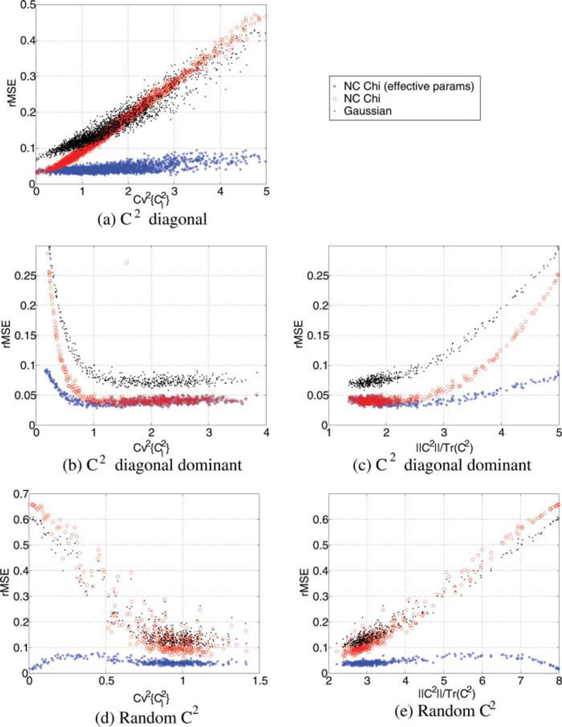
- We will analyze the error committed with the nc-χ2 approximation for different configurations of matrix C2. To avoid any effect of the signal over the noise, we first assume that μi = 0. We define 104 samples of 8 complex Gaussian RVs and a 8 × 8 coefficient matrix W, so that three different scenarios are considered (see Appendix for more details about the relation between matrix C2 configuration and the final distribution):
- Matrix C2 is diagonal (different elements in the diagonal).
- Matrix C2 is not diagonal and the diagonal elements are greater than the rest of the elements (diagonal dominant).
- Matrix C2 is totally random.
- The coefficient of variation of the elements of the diagonal: .
- The ratio between the determinant of C2 and the trace of the matrix: ‖C2‖/Tr(C2). This is a measure of the weight of the non-diagonal elements over the diagonal. Note that for the first case, this parameter is a constant.
where pO(x) is the PDF of the original data (estimated from the histogram of the 104 samples for each pixel) and pz(x) is the distribution to fit.[19] We will test the model fit for different SNR values with a given set of weights. We consider 104 samples of 8 complex Gaussian RVs with unitary variance and mean in the range μ ∈ (0, 3), i.e., ~N(μ, 1). The RVs are combined using 8 × 8 complex random weights (selected in a range similar to an actual GRAPPA reconstruction) and the SoS is considered. We calculate the error of fitting a nc-χ2 and a Gaussian for different SNR values, defining the original SNR in each coil as .
Experiment with the MR Data-Sets
In a second stage, GRAPPA coefficients from actual MR acquisitions will be used. In each case, a rectangular 2 ky - by- 5 kx GRAPPA convolution kernel η(k) is employed. The following experiments are considered:
Data sets 1 and 2: The k–space data are 2× subsampled with 32 ACS lines–skipping every other line except in the central region. From the ACS lines the GRAPPA coefficients ωm(l, k) are estimated. The k–space domain coefficients are then transformed to x-space, Wm(l, x). The experiments proposed for synthetic data are repeated using the calculated GRAPPA coefficients. For each of the pixels in the image we consider 104 samples of 8 complex Gaussian RVs with unitary variance and mean in the range μ ∈ (0, 4), so that original SNR ∈ (0, 4). To simulate the reconstruction process, for each of the values of x the RVS are combined following Eq. 9, and the composite magnitude image is obtained by SoS. For the sake of simplicity, will be used. After reconstruction, 104 samples of the 256 × 256 image are available. The distribution of the data is tested by fitting a theoretical probability distribution to the real data. To that end, the rMSE is measured. The same three distributions used in the synthetic experiments (nc-χ2 with effective parameters, nc-χ2 with the original parameters and Gaussian) are considered.
Data set 1: To further test it, the experiment for Data set 1 is repeated with SNR = 1. A variable number of samples is considered, and a Kolmogorov–Smirnov test at a significance level of α = 0.05 is used to decide whether the sample data follow any of the proposed distributions.
Data set 3: The GRAPPA reconstruction coefficients are derived from one of the 60 samples, using 2× subsampling and 32 ACS lines. All the 60 samples are 2× subsampled and reconstructed with the same GRAPPA coefficients and the composite magnitude image is obtained by SoS. Agolden standard (to obtain the Ai values) is created by averaging the complex data in each coil. The original σn and σK values for each coil are estimated from the background of the fully sampled images (6). Theoretical values of Leff (x) and are calculated for each point x. A Kolmogorov–Smirnov test at a significance level of α = 0.05 is used to decide whether each x point of the 60 samples follow a nc-χ distributions with parameters Leff (x) and .
RESULTS
Synthetic Experiments
First, we will consider the experiments with synthetically generated weights. Results for the first experiment are shown in Fig. 2. Note that the nc-χ2 distribution with effective parameters is the distribution that better follows the actual variations of the data for both experiments. The more asymmetric the distribution, the better is the behavior of the nc-χ2 when compared with the Gaussian.
FIG. 2.
Actual distribution of the SoS of the sum of weighted Normal RVs compared with nc-χ2 distribution approximation and Gaussian distribution. [Color figure can be viewed in the online issue, which is available at wileyonlinelibrary.com.]
The second experiment measures the error of the different approximations as a function of the configuration of matrix C2, i.e., the coefficients. Results are depicted in Fig. 3. In all the cases, the nc-χ2 distribution with effective values is the one that shows a lower rMSE for a wider range of variation of parameters. In all the cases, the error of approximating the actual distribution by a nc-χ2 is always smaller than 0.1, usually around 0.05. In Fig. 3a (diagonal case) we can see that as the values in the diagonal are more different, the Gaussian and the nc-χ2 with original parameters produce a greater error. However, the approximation with effective parameters remains constant. Fig. 3(b–c) shows the results for the dominant diagonal, and Fig. 3(d–e) the results for the random C2. An interesting effect in these two experiments is that for the original nc-χ2 and the Gaussian approaches the error increases when the ratio ‖C2‖/Tr(C2) grows. It means that, as the diagonal becomes less significant, these two approaches are not a good representation of the data. The nc-χ2 approximation with effective parameters due precisely to the fine tune of these effective parameters, is able to properly fit the actual distribution.
FIG. 3.
Relative errors in the PDF for the non-central Chi approximation with effective parameters. For the sake of comparison, the noncentral Chi with fix parameters and the Gaussian distribution are also considered. [Color figure can be viewed in the online issue, which is available at wileyonlinelibrary.com.]
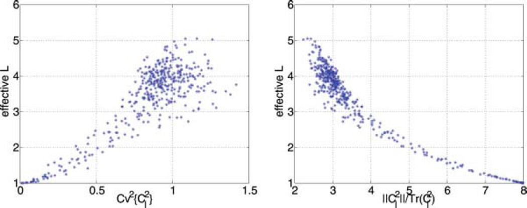
The evolution of the effective number of coils for the experiment in Fig 3(d–e) is reproduced in Fig. 4. As the ratio ‖C2‖/Tr(C2) grows, the correlation between variables also grows. As a consequence, the number of DoF of the system will decrease together with the effective number of coils, Leff. This reduction in Leff implies an increase in and consequently a decrease in the SNR.
FIG. 4.
Evolution of the effective value of parameter L for the experiments in Fig 3(d–e). [Color figure can be viewed in the online issue, which is available at wileyonlinelibrary.com.]
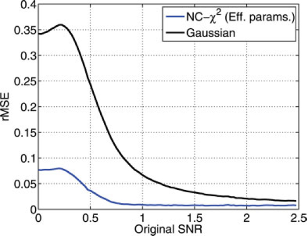
The third synthetic experiment deals with the error of the approximation for different SNR configurations. Results are depicted in Fig. 5. For large SNR values (SNR > 2), the nc-χ2 and the Gaussian approximation converges, as expected.
FIG. 5.
Relative errors for the nc-χ2 approximation with effective parameters and Gaussian for different SNR values. [Color figure can be viewed in the online issue, which is available at wileyonlinelibrary.com.]
Experiment with the MR Data-Sets
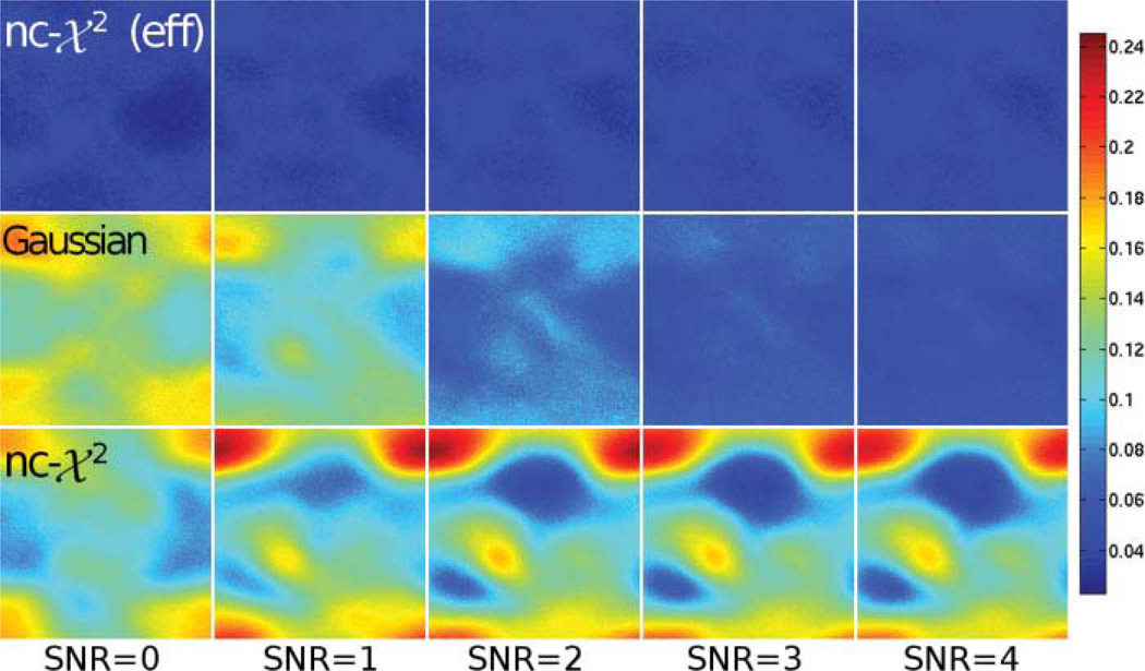
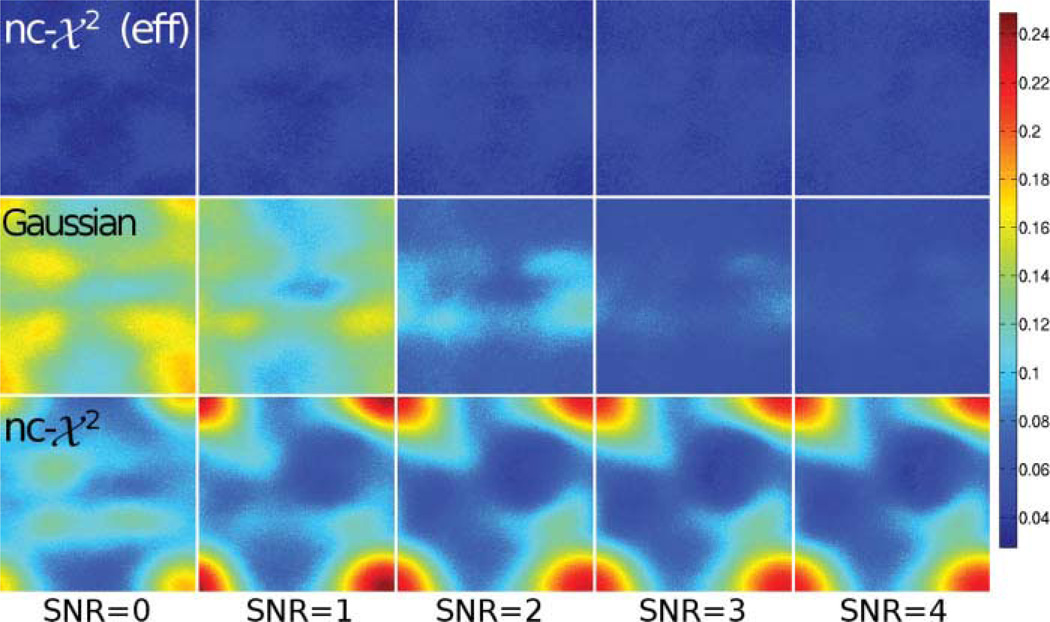
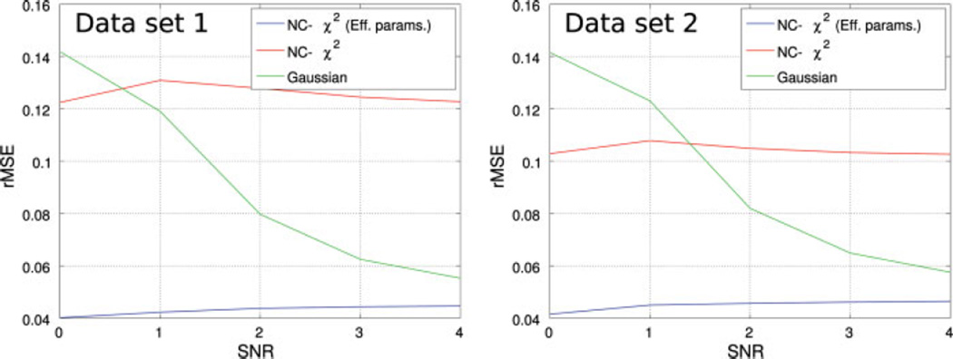
The next step is to analyze the results generated by estimated GRAPPA coefficients. Results for the data fit for different distributions are shown in Fig. 6 for the data set 1 and in Fig. 7 for the data set 2. In both cases, the rMSE for each of the points of the final image is shown. For better illustration, the average of the rMSE in the whole image is depicted in Fig. 8. Regardless of the SNR level, the error committed when approximating the distribution by a nc-χ2 with effective parameters is always lower than 6%, while the other two models (Gaussian and nc-χ2) show greater values. What is more, the rMSE for nc-χ2 is quite independent of the SNR value. As expected, the Gaussian model is a good approximation when SNR increases. On the other hand, if nc-χ2 is considered but the effective parameters are not used, the error even increases together with the SNR in certain areas of the image.
FIG. 6.
rMSE of different statistical approximations using the GRAPPA coefficients of dataset 1. Different original SNR are considered. Top row: nc-χ2 with effective parameters. Middle row: Gaussian. Bottom row: nc-χ2 with original parameters. [Color figure can be viewed in the online issue, which is available at wileyonlinelibrary.com.]
FIG. 7.
rMSE of different statistical approximations using the GRAPPA coefficients of dataset 2. Different original SNR are considered. Top row: nc-χ2 with effective parameters. Middle row: Gaussian. Bottom row: nc-χ2 with original parameters. [Color figure can be viewed in the online issue, which is available at wileyonlinelibrary.com.]
FIG. 8.
Average of the rMSE in the whole image for the different SNR values.
From these results, we can conclude that the nc-χ model (with effective parameters) proposed gives a small error when considering the GRAPPA reconstruction coefficients from actual parallel acquisitions.
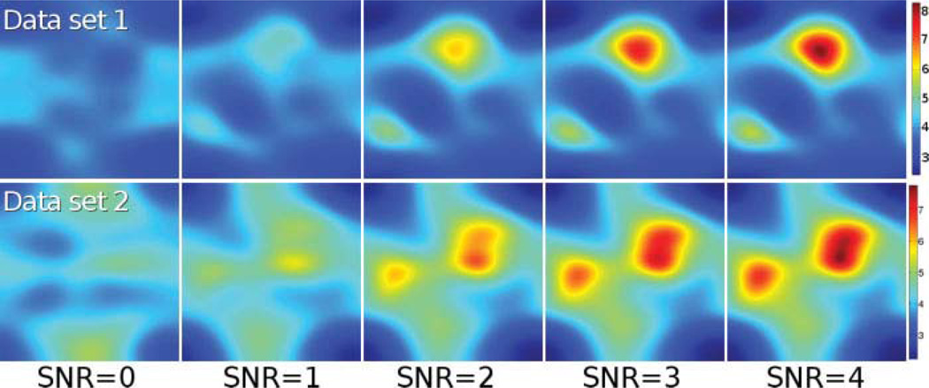
It is also interesting analyzing the distribution of the effective parameters along the image. Note that these parameters only depend on the GRAPPA coefficients. The effective number of coils (Leff) is shown in Fig. 9 and the effective variance of noise is shown in Fig. 10. Note that those cases with low SNR also show low levels of the effective number of coils. Note also that the distribution of Leff correlates with the error committed when considering nc-χ2 without effective parameters. The points with lower rMSE are logically those with greatest values of Leff.
FIG. 9.
L effective for different SNR values. Top: Data set 1. Bottom: Data set 2.
FIG. 10.
σn effective for different SNR values. Top: Data set 1. Bottom: Data set 2.
The variance of noise, on the other hand, shows a great variation along the image, which confirms the non-stationarity assumption previously done. Values of σn range between 2 and 6. However, note that the variation of this parameter across the image is soft. So, in some applications (like filtering methods) local stationarity may be assumed if needed.
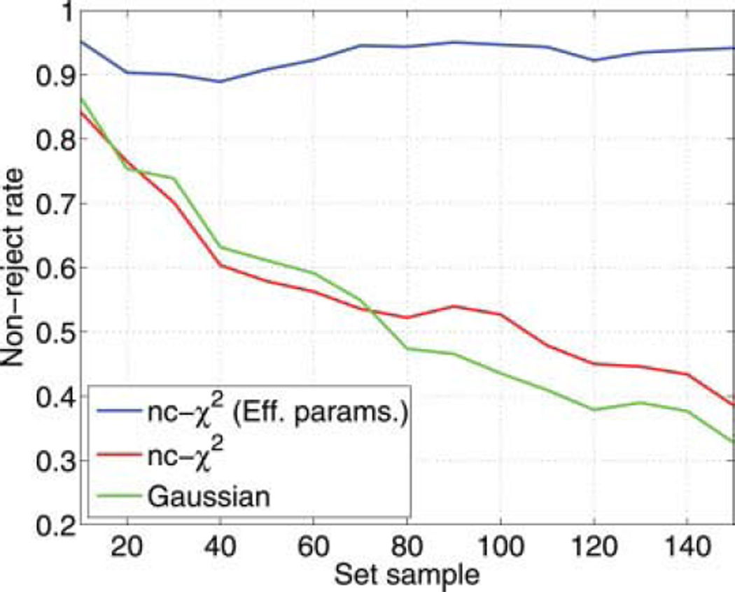
In Fig. 11, the acceptance rate by the Kolmogorov-Smirnov test for different set sizes is depicted. The acceptance rate for the nc-χ2 model (with effective parameters) is over the 90% even for large population sizes. The larger the size of the sample, the easier for the test to reject the null hypothesis. For the Gaussian and nc-χ2 models, the rate goes down very fast, so that they can only be accepted for very small populations. It may be concluded that the effective nc-χ2 model accurately fits data generated following the GRAPPA reconstruction algorithm.
FIG. 11.
Rate of sets passing the Kolmogorov–Smirnov test for the distributions under study as a function of the size of the population. Significance level is α = 0.05, and a SNR = 1. The data are synthetically generated from the GRAPPA coefficients of data set 1. [Color figure can be viewed in the online issue, which is available at wileyonlinelibrary.com.]
Finally, the Kolmogorov-Smirnov test is run over the 60 GRAPPA reconstructed samples of the MR phantom (data set 3). The 90.13% of the points in the image passed the test, which correlates well with the results of the previous experiment, and confirms the nc-χ (with effective parameters) as a suitable distribution to accurately model data after GRAPPA reconstruction and SoS.
DISCUSSION
The statistical characterization of the composite magnitude signal after GRAPPA reconstruction as a parameterized non–stationary nc-χ distribution has been derived. In fully sampled images, the derivation of the magnitude signal distribution is a straight transformation from the prior Gaussian model for each coil. With pMRI techniques, the final model strongly depends on the particular algorithm used. In general, those reconstructing one single image domain drive to a Rician distribution, since the magnitude is computed as the modulus of a Gaussian variable. Contrary to conventional MRI, the noise in the image cannot be considered stationary strictly speaking, since its variance shows fluctuations across the image. Besides, noisy samples cannot be considered independent either, due to interpolation artifacts.
The analysis of GRAPPA reconstructed signals is more difficult. Although its feature of providing one complete image domain for each receiving coil assimilates it to conventional multiple coils systems, the non–central Chi distribution does not directly apply to this case. Apart from the aforementioned interpolation artifacts related to non–stationary noisy patterns and correlations, the noise variance for each receiving coil is different with this kind of reconstruction. Hence, a non–central Chi model cannot be assumed in general. For brain images, which are the data sets of interest in this dissertation, it has been shown that in fact this distribution is a very accurate approximation to the actual statistics of noise. However, as a consequence of the correlation between the reconstructed data in each coil, reduced effective parameters, namely the effective number of coils and the effective variance of noise, must be taken into account. Thus, the final distribution for each point is equivalent to an acquisition with a fewer number of coils and a greater variance of noise.
We want to remark the importance of the suitable statistical model for GRAPPA proposed here. As an example. we will propose some future applications. (1) In the case of tensor estimation in DTI, in (11) authors show that weighted least squares is theoretically a good method to estimate the DT if the data is nc-χ distributed. GRAPPA reconstructed data is being widely used for these purposes, but knowing the models we assure a good estimation, and we can measure the bias and variance of the estimation error. (2) Although the signal is non-stationary, we can assume a small spatial variation of the parameters. This way, we can calculate local statistics and reformulate Rician noise filtering methods, like the conventional approach (1), ML (2), or LMMSE (3). These algorithms will need as an input the number of coils L and the variance of noise . When applied over GRAPPA images, the new derived effective parameters must be used instead. (3) Noise estimation is usually done assuming that the noise is stationary in the background (26), i.e., the value of the variance of noise is homogenous for all the pixels in the background. As a consequence, those methods cannot be directly applied with GRAPPA. However, with the effective σn value derived for each x value in the image, the inhomogeneous background in GRAPPA can be easily corrected and used for estimation, straightly applying some of the methods in (6).
It is also convenient to stress the limitations of the study performed in this paper. First, the analysis carried out in this article is only valid for the SoS to combine the images from each coil. Other methods used by newer systems, such as linear channel combination or B1 maps have not been considered. With these methods Eq. 14 will differ, and a new study of parameters will be needed. Finally, certain MRI techniques, such as EPI, which can show their own peculiarities with regard to the statistical characterization of noise, has been removed from the study.
CONCLUSIONS
The main contribution of this article is the statistical characterization of the composite magnitude signal after GRAPPA reconstruction as a parameterized non–stationary nc-χ distribution. We have shown that although data does not strictly follows a non–central Chi model, in practical cases this distribution is a very accurate approximation to the actual statistics of noise in the magnitude composite signal when SoS is used. To really fit the distribution to the data, reduced effective parameters are considered: the effective number of coils and the effective variance of noise. As a final remark, we want to point out that the studied carried out is totally valid if initial correlations are assumed between coils.
Acknowledgments
Grant sponsor: Junta de Castilla y León; Grant numbers: SAN126/VA33/09, VA0339A10-2; Grant sponsor: Consejería de Sanidad de Castilla y León; Grant number: GRS 292/A/08; Grant sponsors: NIH U41 RR-019703 (PI:Jolesz) and the Functional Neuroimaging Lab at Brigham and Women’s Hospital, Boston, MA
APPENDIX
About the SoS of the Sum of Weighted Normal Variables
Let , l = {1, …, L}, be a set of independent Gaussian complex RVs with mean μl and variance . For simplicity, let us initially assume a diagonal covariance matrix, i.e. there is not any initial correlation between variables:
We define a linear combination of these RVs (as the one done for each pixel in GRAPPA in the x-space, see Eq. 8) using complex weights as
with Wil a set of known (generic) complex weights which are arranged into the following matrix:
| [20] |
The (square) sum of squares (SoS) is defined as:
| [21] |
| [22] |
with
Note that . Let us define matrix C2 as
There are three possible scenarios directly related to the three requirements for the nc-χ described in section “Statistical model in single- and multiple-coil MR signals”:
- Matrix C2 is diagonal and with all the elements in the diagonal equal and the variance of all the Gaussian variables is the same, i.e., . All the requirements are fulfilled and X2 follows a non-central Chi square (nc-χ2) distribution (27) with PDF:
with and . The mean and the variance of the distribution will be[23] [24] [25] - Matrix C2 is diagonal, but the variance of each variable is different, and therefore the elements of the diagonal are different. In this case, the second requirement is not fulfilled and the distribution of X2 is no longer nc-χ2. For each variable, |Mi|2 will follow a nc-χ2 distribution as the one in Eq. 23 with L = 1 and its characteristic function will be
Therefore, the characteristic function for X2 will become:
The mean and the variance of this distribution are:[26]
The greater the fluctuation of the noise power along the coils, the greater the error committed when approximated by a nc-χ2. The error in the approximation can be measured by the variability of .[27] - Matrix C2 is not diagonal. Neither the second nor the third requirements are fulfilled. In this case, the final PDF or the characteristic function become hard to derive theoretically. The mean and the variance can be calculated:
[28]
with[29]
If we define the covariance matrix of X2 as (24)
the mean and the variance can be rewritten as[30] [31]
with ‖․‖F the Frobenious norm and A = [A1, A2, …, AL]T.[32]
The third case is the one usually found when dealing with GRAPPA reconstruction. As an effect of the correlation between the RVS Mi, the number of DoF of the final distribution would decrease. To fit the new distribution to a nc-χ2, the method of the moments is used over the theoretical mean and variance in Eqs. 24, 25, 28, and 29. As a result, the final nc-χ2 shows new effective values for the parameters L and σ:
| [33] |
| [34] |
The effective L parameter is directly related to the DoF of the distribution, and it will decrease. As a consequence, parameter σ will increase.
This solution has been obtained assuming that there is no initial correlation between coils. However, it can be easily extrapolated to the correlated case. Note that even if Σ2 is not diagonal, it is an Hermitian, positive-definite matrix, and therefore it can be decomposed as:
with D the real, diagonal matrix with positive eigenvalues. Thus, we can write:
So, although Σ2 is not diagonal, we can decorrelate it by assuming an effective weight matrix We = WU and an effective decorrelated initial covariance matrix . The final covariance matrix will be
With this formulation, results in Eqs. 33–34 are totally valid for the correlated case.
Footnotes
Note that since Ai = 0, we are really fitting a central χ2 rather than a nc-χ2, but the reasoning and the conclusions are similar.
REFERENCES
- 1.McGibney G, Smith M. Unbiased signal-to-noise ratio measure for magnetic resonance images. Med Phys. 1993;20:1077–1078. doi: 10.1118/1.597004. [DOI] [PubMed] [Google Scholar]
- 2.Sijbers J, den Dekker AJ, Van Dyck D, Raman E. Estimation of signal and noise from Rician distributed data. Proc. of the Int. Conf. on Signal Proc. and Comm.; Las Palmas de Gran Canaria, Spain. 1998. pp. 140–142. [Google Scholar]
- 3.Aja-Fernández S, Alberola-López C, Westin CF. Noise and signal estimation in magnitude MRI and Rician distributed images: a LMMSE approach. IEEE Trans Image Proccess. 2008;17:1383–1398. doi: 10.1109/TIP.2008.925382. [DOI] [PubMed] [Google Scholar]
- 4.Wiest-Daesslé N, Prima S, Coupé P, Morrissey S, Barillot C. Rician noise removal by non-local means filtering for low signal-to-noise ratio MRI: Applications to DT-MRI. Lecture Notes in Computer Science, MICCAI 2008. 2008:171–179. doi: 10.1007/978-3-540-85990-1_21. [DOI] [PMC free article] [PubMed] [Google Scholar]
- 5.Constantinides C, Atalar E, McVeigh E. Signal-to-noise measurements in magnitude images from NMR based arrays. Magn Reson Med. 1997;38:852–857. doi: 10.1002/mrm.1910380524. [DOI] [PMC free article] [PubMed] [Google Scholar]
- 6.Aja-Fernández S, Tristán-Vega A, Alberola-López C. Noise estimation in single- and multiple-coil magnetic resonance data based on statistical models. Magn Reson Imaging. 2009;27:1397–1409. doi: 10.1016/j.mri.2009.05.025. [DOI] [PubMed] [Google Scholar]
- 7.Sijbers J, den Dekker A, Van Audekerke J, Verhoye M, Van Dyck D. Estimation of the noise in magnitude MR images. Magn Reson Imaging. 1998;16:87–90. doi: 10.1016/s0730-725x(97)00199-9. [DOI] [PubMed] [Google Scholar]
- 8.Brummer M, Mersereau R, Eisner R, Lewine R. Automatic detection of brain contours in MRI data sets. IEEE Trans Med Imaging. 1993;12:153–166. doi: 10.1109/42.232244. [DOI] [PubMed] [Google Scholar]
- 9.Sijbers J, Poot D, den Dekker AJ, Pintjenst W. Automatic estimation of the noise variance from the histogram of a magnetic resonance image. Phys Med Biol. 2007;52:1335–1348. doi: 10.1088/0031-9155/52/5/009. [DOI] [PubMed] [Google Scholar]
- 10.Salvador R, Peña A, Menon DK, Carpenter T, Pickard J, Bullmore ET. Formal characterization and extension of the linearized diffusion tensor model. Hum Brain Mapp. 2005;24:144–155. doi: 10.1002/hbm.20076. [DOI] [PMC free article] [PubMed] [Google Scholar]
- 11.Tristán-Vega A, Westin CF, Aja-Fernández S. MICCAI 2009, Lecture Notes in Computer Science. vol. 5761. New York: Springer; 2009. Bias of least squares approaches for diffusion tensor estimation from array coils in DT–MRI; pp. 919–926. [DOI] [PMC free article] [PubMed] [Google Scholar]
- 12.Fillard P, Pennec X, Arsigny V, Ayache N. Clinical DT-MRI estimation, smoothing, and fiber tracking with log-Euclidean metrics. IEEE Trans Med Imaging. 2007;26:1472–1482. doi: 10.1109/TMI.2007.899173. [DOI] [PubMed] [Google Scholar]
- 13.Gudbjartsson H, Patz S. The Rician distribution of noisy MRI data. Magn Reson Med. 1995;34:910–914. doi: 10.1002/mrm.1910340618. [DOI] [PMC free article] [PubMed] [Google Scholar]
- 14.Hoge WS, Brooks DH, Madore B, Kyriakos WE. A tour of accelerated parallel MR imaging from a linear systems perspective. Concepts Magn Reson Part A. 2005;27A:17–37. [Google Scholar]
- 15.Larkman DJ, Nunes RG. Parallel magnetic resonance imaging. Phys Med Biol. 2007;52:15–55. doi: 10.1088/0031-9155/52/7/R01. (Invited Topical Review). [DOI] [PubMed] [Google Scholar]
- 16.Pruessmann KP, Weiger M, Scheidegger MB, Boesiger P. SENSE: sensitivity encoding for fast MRI. Magn Reson Med. 1999;42:952–962. [PubMed] [Google Scholar]
- 17.Griswold MA, Jakob PM, Heidemann RM, Nittka M, Jellus V, Wang J, Kiefer B, Haase A. Generalized autocalibrating partially parallel acquisitions (GRAPPA) Magn Reson Med. 2002;47:1202–1210. doi: 10.1002/mrm.10171. [DOI] [PubMed] [Google Scholar]
- 18.Dietrich O, Raya J, Reeder SB, Ingrisch M, Reiser M, Schoenberg SO. Influence of multichannel combination, parallel imaging and other reconstruction techniques on MRI noise characteristics. Magn Reson Imaging. 2008;26:754–762. doi: 10.1016/j.mri.2008.02.001. [DOI] [PubMed] [Google Scholar]
- 19.Thünberg P, Zetterberg P. Noise distribution in SENSE- and GRAPPA-reconstructed images: a computer simulation study. Magn Reson Imaging. 2007;25:1089–1094. doi: 10.1016/j.mri.2006.11.003. [DOI] [PubMed] [Google Scholar]
- 20.Gudbjartsson H, Patz S. The Rician distribution of noisy MRI data. Magn Reson Med. 1995;34:910–914. doi: 10.1002/mrm.1910340618. [DOI] [PMC free article] [PubMed] [Google Scholar]
- 21.Liang ZP, Lauterbur PC. Principles of magnetic resonance imaging. A signal processing perspective. New York: IEEE Press; 2000. [Google Scholar]
- 22.Roemer P, Edelstein W, Hayes C, Souza S, Mueller O. The NMR phased array. Magn Reson Med. 1990;16:192–225. doi: 10.1002/mrm.1910160203. [DOI] [PubMed] [Google Scholar]
- 23.Blaimer M, Breuer F, Mueller M, Heidemann R, Griswold M, Jakob P. SMASH, SENSE, PILS, GRAPPA: how to choose the optimal method. Top Magn Reson Imaging. 2004;15:223–236. doi: 10.1097/01.rmr.0000136558.09801.dd. [DOI] [PubMed] [Google Scholar]
- 24.Breuer FA, Kannengiesser SA, Blaimer M, Seiberlich N, Jakob PM, Griswold MA. General formulation for quantitative g-factor calculation in grappa reconstructions. Magn Reson Med. 2009;62:739–746. doi: 10.1002/mrm.22066. [DOI] [PubMed] [Google Scholar]
- 25.Ji JX, Son JB, Rane SD. PULSAR: A matlab toolbox for parallel magnetic resonance imaging using array coils and multiple channel receivers. Concepts Magn Reson Part B Magn Reson Eng. 2007;31B:24–36. [Google Scholar]
- 26.Haacke EM, Brown RW, Thompson MR, Venkatesan R. Magnetic resonance imaging: physical principles and sequence design. New York: John Wiley and Sons; 1999. [Google Scholar]
- 27.Simon MK. Probability distributions involving Gaussian random variables. Norwell, MA: Kluwer Academic Publishers; 2002. [Google Scholar]


