

Abstract
We present a preliminary test of the Ensemble Optimal Statistical Interpolation (EnOSI) method for the statistical tracking of an emerging epidemic, with a comparison to its popular relative for Bayesian data assimilation, the Ensemble Kalman Filter (EnKF). The spatial data for this test was generated by a spatial susceptible-infectious-removed (S-I-R) epidemic model of an airborne infectious disease. Both tracking methods in this test employed Poisson rather than Gaussian noise, so as to handle epidemic data more accurately. The EnOSI and EnKF tracking methods worked well on the main body of the simulated spatial epidemic, but the EnOSI was able to detect and track a distant secondary focus of infection that the EnKF missed entirely.
Keywords: Bayesian statistical tracking, emerging epidemics, spatial S-I-R epidemic model, data assimilation, ensemble Kalman filter, optimal statistical interpolation
1. Introduction
Mathematical models have been used since 1927 to describe the rise and fall of infectious disease epidemics (Diekmann and Heesterbeek, 2000; Castillo-Chávez and Blower, 2002a,b; Ma and Xia, 2009). A majority of the models are variations of the three-compartment nonlinear Susceptible-Infectious-Removed (S-I-R) model developed by Kermack and McKendrick (1927). A person occupies the susceptible or infectious compartments if he or she can contract or transmit the disease, respectively. The removed compartment includes those who have died, have been quarantined, or have recovered from the disease and become immune. The state variables are the number of susceptible (S), the infectious (I), and the removed (R) in a closed population. S-I-R models often perform surprisingly well in modeling the temporal evolution of real-world epidemics, and their spatial variants can produce a traveling-wave spatial dynamic similar to that displayed by some epidemics. Here the infectious population is in the crest of the wave, with the susceptible population in front of the crest, leaving the removed behind.
Tracking and forecasting the full spatio-temporal evolution of an emerging epidemic is notoriously difficult. Often observational data may be affected by many sources of measurement error, new data arrives on an irregular schedule, and the model itself is incorrect in unknown ways. These are also well-known problems in a variety of empirical areas of high importance, such as storm and wildfire forecasting. The general category of statistical tracking techniques that incorporate error-prone data as they arrive by sequential statistical estimation is known as data assimilation (Kalnay, 2003). Use of the statistical methods of data assimilation can increase the accuracy and reliability of epidemic tracking by incorporating data as it arrives, with weighting factors that reflect the observed or expected reliability of the observations. A few applications of data assimilation in epidemiology already exist (Kalivianakis et al., 1994; Cazelles and Chau, 1997; Costa et al., 2005; Bettencourt et al., 2007; Bettencourt and Ribeiro, 2008; Jégat et al., 2008; Rhodes and Hollingsworth, 2009; Dukic et al., 2009; Mandel et al., 2010a; Angulo et al., 2012; Shaman et al., 2013).
The goal of this study is to conduct a preliminary test of the ensemble optimal statistical interpolation (EnOSI) tracking method, including a comparison with a closely related tracking technique known as the ensemble Kalman filter (EnKF). The EnKF and other ensemble-based data assimilation methods are already popular in meteorology and oceanography, where the dimensionality of the state space commonly exceeds one million cells. When coupled with a spatial dynamic model, these methods can be used to forecast the spatio-temporal evolution of an epidemic, and to adjust those forecasts appropriately as sparse and error-prone data arrives.
This paper is organized as follows. In Section 2 we present a stochastic spatial epidemic model, and we use it to generate data for the spatial spread of an infectious disease. In Section 3, we illustrate the Bayesian tracking of emerging epidemics using EnOSI with a simulated epidemic wave originating in Santa Fe, New Mexico. In Section 4, we compare the EnOSI tracking results for the stochastic spatial epidemic model with the EnKF variant presented in Section 3. Finally, in Section 5, we summarize the computational efforts and discuss the significant challenges in implementing the discussed methods. We provide some concluding remarks and future directions.
2. A Stochastic Spatial Epidemic Model
2.1. Epidemic Dynamics
For this study we use a discretized stochastic version of the Hoppensteadt (1975) spatial S-I-R epidemic model. As with almost all spatial epidemic models since Bailey (1957, 1967) and Kendall (1965), we assume that individuals are continuously distributed on a spatial domain. This model uses three variables to define the state of the epidemic at each (x, y) coordinate:
S(x, y, t) = density (per unit area) of the susceptible population,
I(x, y, t) = density of the infectious population, and
R(x, y, t) = density of the removed population.
Thus, each of these variables is a scalar field that evolves with time. In continuous time the epidemic dynamics are defined by a system of three partial differential equations for the state variables. The population is considered to be dispersed over a connected planar domain ; its density is a function of the spatial coordinates x and y. There are no vital dynamics in this model, meaning that there are no new births or non-disease-related deaths in any of the three compartments, and there are no movements of the population. The (deterministic) evolution of the state (S (t) , I (t) , R (t)) is given by
| (1) |
The function q (x, y, t) gives the rate of removal of infectives due to death, quarantine, or recovery with immunity. The weight function w (x, y, u, v) measures the influence of infectives at spatial position (u, v) on the exposure of susceptibles at position (x, y); in this simulation we used the kernel function w (x, y, u, v) = α exp[−((x – u)2 + (y – v)2)1/2/λ], which expresses the idea that the influence of nearby infectives drops off as an exponential function of Euclidean distance, with constant λ, a characteristic of the distance at which the disease spreads. More mobile societies will have larger values of λ. The parameter α measures the infectiousness of the disease, given by the product of mixing rate and the infection rate.
The simulation evolves on a two-dimensional discretized spatial domain with a total of p = n × m grid cells. A stochastic cell model is created by treating the quantities on the right-hand-side of (1) as the intensities of a Poisson process and by piecewise constant integration over the cells. The domain Ω is decomposed into nonoverlapping cells Ωi with centers (xi, yi) and areas A (Ωi), i = 1, … , p. The state in the inhabitable cell Ωi is the random element (Si, Ii, Ri), advanced in time over the interval [t, t + Δt] by
where the random increments ΔSi and ΔRi are sampled from
| (2) |
The summation in (2) is done only over the cells Ωj near Ωi; for far away cells, the weights w (xi, yi, xj, yj) are negligible (the definition of “near” and “far” depends upon the value of λ). It is not necessary to compute a Poisson-distributed transmission rate from each source cell to a given target cell, because a finite sum of independent Poisson-distributed random variables, each with its own intensity parameter, is itself Poisson-distributed with an intensity parameter equal to the sum of the individual intensities.
Thus a susceptible individual, at a particular location, may become infected when he/she comes in contact with an infectious individual from within a neighboring area, with a monotonically decreasing weighting function that declines exponentially with distance. If this contact causes sufficient secondary infections then a new epidemic focus will develop at that new location.
3. Statistical Tracking Using Data Assimilation Methods
We use data assimilation for the statistical tracking of emerging epidemics as they are unfolding. This involves two basic components: a dynamic model to forecast the state of the epidemic between arrivals of new data, and observations that are used to update an ensemble of state estimates. Data assimilation requires estimating the uncertainty both for model and observations forecasts. Our goal in this paper is to incorporate sparse, episodic and noisy observational epidemic data over space and time into a dynamic statistical model so as to produce an optimal Bayesian estimate of the current spatial distribution of the infectious population, and to forecast the progress of the real epidemic.
3.1. The Kalman Filter (KF)
The Kalman Filter (KF) was first presented by Kalman (1960) and Kalman and Bucy (1961) as a method for tracking the state of a linear dynamic system perturbed by Gaussian white noise. For the Kalman filter in discrete time and space, this means that the errors are drawn from a zero-mean Gaussian distribution with diagonal covariance matrix. The Kalman filter provides a foundation on which to build a Bayesian data assimilation scheme for epidemics, after suitable modifications that allow it to work with the nonlinearities implicit in epidemic dynamics, and with the non-Gaussian nature of epidemic forecasting errors.
The full state of a discretized spatial epidemic model is a grid of n × m cells, each of which contains a characterization of the population currently within the limits of the cell. To apply the Kalman filtering method, we represent the n × m values of the Infectious variable on this grid as a single long vector x with p = n × m elements, which for the purposes of data assimilation is the dimensionality of the state space. If we could observe this state vector without error, our observations would be another vector y that satisfies y = Hx where H is the linear operator that maps the state vector onto the observational space. Now consider the situation in which we have a forecast of the current state, xf, and a newly arrived vector of noisy observations y = Hx + ε, where ε ~ N (0, R). We need to update the forecast by optimally assimilating these new observations. The result will be called the analysis estimate of state, xa. The superscripts f and a are used to denote the forecast (prior) and analysis (posterior) estimate of the current state, respectively.
In the classical Kalman filter, the underlying dynamics are assumed to be linear, e.g.
where F is the matrix of the linear transformation of xt–1 to xt. In other words, it is the model of the dynamic process assumed by the standard Kalman filter. The analysis estimate of the state vector is calculated from
where
Here Kt is the Kalman gain matrix at time t, is the covariance matrix for the forecast state vector, is the covariance matrix for the analysis state vector, and R is the measurement error covariance matrix.
The KF algorithm requires storing and updating the entire covariance matrix of the state vector. In high-dimensional 2D or 3D tracking problems, the storage space required for the covariance matrix may easily exceed any physical storage system. To see the storage problem, consider a 2D simulation of a scalar field that has been discretized on a 103 × 103 grid. The state vector of this system has 106 elements, and its covariance matrix has 106 × 106 = 1012 elements, requiring four terabytes just to store.
The extended Kalman filter (EKF) (Julier et al., 1995) was an early attempt to adapt the basic KF equations for nonlinear problems, through linearization. However, the EKF has its own disadvantages: if the model is strongly nonlinear at the time step of interest, linearization errors can turn out to be non-negligible, which leads to filter divergence (Evensen, 1992). The EKF is not suitable for high-dimensional 2D and 3D data assimilation problems, because it suffers from the same storage requirements as the KF.
Other commonly used Bayesian tracking techniques for nonlinear problems include the unscented Kalman filter (UKF) and the particle filter (PF) (Gordon et al., 1993). Particle filtering is a versatile Monte Carlo technique that can handle nonlinearities in the model and represents the Bayesian posterior probability density function by a set of samples drawn at random with associated weights.
3.2. Ensemble Kalman Filter (EnKF)
The EnKF solves this storage-and-retrieval problem by (in effect) calculating the covariances from the members of an ensemble of simulations, as they are needed. The result is an elegant Bayesian update algorithm with dramatically improved efficiency and storage requirements (Mandel et al., 2010a).
The ensemble Kalman filter (EnKF) was introduced by Evensen (1994), modified to provide correct covariance by Burgers et al. (1998), and improved by Houtekamer and Mitchell (1998). The EnKF is a popular sequential Bayesian data assimilation technique that uses a collection of almost-independent simulations (known as an ensemble) to solve the covariance problem of Kalman filtering for systems with very high-dimensional state vectors. It does this using a two-step process: first estimate the covariance matrix from the ensemble, then perform an ensemble update. The stored covariance matrix of the KF is replaced by sample covariances computed from the ensemble members. These sample covariances are then used to calculate the Kalman gain matrix.
The success of the EnKF in many diverse applications has also stimulated the invention of a plethora of variant algorithms. At our last count, there were at least 15 different named variants of the EnKF in the literature. However, it may be fair to say that there are only two basic approaches to the EnKF update: stochastically perturbed observations (Monte Carlo), and “square-root” filters (deterministic). Both approaches adopt the same covariance estimate step, but differ in the ensemble update step. Regardless of the specific approach employed, the goal is to obtain a Bayesian estimate of the state as efficiently as possible. In many real-world examples these two approaches perform quite similarly. A more detailed description EnKF may be found in the book by Evensen (2009), and there is a good tutorial by Mandel (2007).
The EnKF analysis update equations are the same as the classical KF equations, except that they use the covariance of the forecast ensemble to substitute for the matrix Q, which in a high-dimensional system is, as noted above, too large to store. Let X be a random ensemble matrix of dimension 3p × N whose columns are realizations sampled from the prior distribution of the system state of dimension p = n × m with ensemble size N. Then the EnKF update formula is:
| (3) |
where Y is the observed ensemble data matrix of dimension 3p × N whose columns are the true state perturbed by random Gaussian error. H is, as before, the linear operator that maps the state vector onto the observational space of dimension 3p × 3p. The deviation Y – HXf is commonly referred to as the “observed-minus-forecast residual” or simply as the innovation. In the above equation Ke is the ensemble Kalman gain matrix given by
where Qf is the forecast-error covariance matrix of dimension 3p × 3p, and R is the symmetric and positive-definite observational (measurement) error covariance matrix of dimension 3p × 3p. The EnKF technique contains two sources of randomness: the random model input, and the measurement errors. Assuming that these two sources of randomness are uncorrelated, the analysis-error covariance matrix of dimension 3p × 3p can be computed from the equation
3.3. Ensemble Optimal Statistical Interpolation (EnOSI)
In the EnKF, the model error covariance matrix is evolved fully at each data assimilation step using an MCMC method. In contrast, Optimal Statistical Interpolation (OSI) is a data assimilation technique based on statistical estimation theory in which the model error covariance matrix is predetermined and assumed to be time-invariant. The model error covariance matrix is dependent only on the distance between spatial grid cells. The correlation length can be adjusted empirically.
OSI was derived by Eliassen (1954). This method has been referred to as “Statistical Interpolation”, “Optimal Interpolation”, or “Objective Analysis.” OSI is called univariate if the observations are of a single scalar field, and multivariate if the observations of one or more scalar fields are used for estimating another scalar field (Talagrand, 2003). Multivariate OSI was developed independently by Gandin (1965) for the analysis of meteorological fields in the former Soviet Union. It requires the specification of the cross-covariance matrix between the observed scalar fields and the scalar field to be estimated (Borovikov et al., 2005).
The ensemble OSI (EnOSI), used here, requires less computational effort than the EnKF, because the model error covariance matrix is fixed and not recalculated at every update step. The EnOSI approach may provide a practical and cost-effective alternative to the EnKF for tracking epidemics. The constant model error covariance matrix in our epidemic simulation used a version with the covariance function having an exponential decay along the off-diagonal entries. The ensemble Kalman gain matrix was then calculated using this time-invariant covariance matrix with a fixed structure, but its spatial structure is derived from an ensemble of state vectors. The accuracy of the EnOSI process will be affected if the approximate covariance matrix differs substantially from the true covariance matrix. Therefore, one disadvantage of the EnOSI is the need for a fixed spatial covariance structure that can reasonably represent the epidemic dynamics throughout the whole domain at all times.
The EnOSI analysis update equation, using the constant covariance, is given by
| (4) |
where
3.4. Example: An Epidemic Wave Originating In New Mexico
To create a preliminary test of the performance of EnOSI and other tracking algorithms designed for high-dimensional state vectors, we constructed a spatial simulation of an epidemic that originates in Santa Fe, New Mexico, and spreads outwards towards Albuquerque and Denver, Colorado. In this simulation the epidemic moves smoothly towards Albuquerque, but jumps suddenly to Denver as if carried by an infectious traveler in an automobile or airplane. Properly detecting and assimilating a new locus of infection that is far from any existing loci is a serious challenge for EnKF algorithms (Beezley and Mandel, 2008; Mandel et al., 2010a). Unlike the EnKF, the EnOSI handles such situations without difficulty.
To improve the realism of the test for the case in which an entirely new disease emerges for the first time, we initialized all members of the tracking ensemble so that they contain no disease whatsoever. New observations in the form of an empirical scalar field of disease prevalence arrives at time steps 10, 20, 30, 40, and 50. These data are complete in the sense that in this case H is just the identity matrix (i.e. there is no regional aggregation of data, and no missing data). The tracking algorithm forecasts the state up until the time when data is received, and then it assimilates this data into the forecast.
The R statistical computing language (R Development Core Team, 2010), freely available from www.cran.r-project.org , was used to carry out the simulations for the spatial spread of the epidemic. Population density data were downloaded as Gridded Population of the World (GPW) data files for 2010 at 1/4 degree resolution from the Center for International Earth Science Information Network at the Columbia University (CIESIN, 2002) and converted to the array-oriented Network Common Data Form (NetCDF) format. High resolution files are preferred for regional subsets. The 1/2 degree GPW resolution was too coarse, and the 2.5 minute GPW resolution generated a covariance matrix that was too large for storage in a laptop computer. We settled on the 1/4 degree GPW resolution as a compromise. We restricted the simulation to the rectangle defined by the coordinates: West: −109°, East: −102°, North: 41.2°, South: 31.4°. These datasets were then loaded into R using the built-in package ncdf (Pierce, 2010).
4. Results
We have applied the EnOSI for the New Mexico-Colorado example mentioned above to the epidemic model described in Section 2 with an ensemble of size 25. We have found as an empirical matter that an ensemble of just 25 members works almost as well as 100 or more members for the EnOSI, but we have not performed any systematic set of tests such as described by Gillijns et al. (2006). The asymptotics of the EnOSI will have to be found analytically, with a convergence proof such as the one we constructed earlier for the EnKF (Mandel et al., 2011). For this example the Infectious state of the model is the output of the observation function. Synthetic data were simulated from a model and initialized in exactly the same way as the ensemble.
In our epidemic application, the perturbed observations Y in (3) and (4) were obtained by sampling from the Poisson distribution with the intensity equal to the data value, instead of using Gaussian perturbations as in the standard EnKF. This is the key feature behind the successful use of our method and it also guarantees that Y has nonnegative entries and thus the columns of Y are meaningful as the Infectious variable.
The result for each member of the ensemble is a Bayesian update of the forecast scalar field, which is referred to as the analysis (i.e. the posterior estimate). We assume that data arrive only once every 10 time steps, with errors. A total of 5 assimilation cycles were performed in this manner. The mean and standard deviation (not reported here) of the ensemble analysis values in each cell of the scalar field gives the EnOSI estimate of the state of the epidemic, with its uncertainty quantified. The following figures present a spatial “image” of the number of infectious persons over the planar domain considered in the New Mexico-Colorado example. All images were generated using NASA Panoply software (Schmunk, 2013) from NetCDF input.
Figure 2 shows the epidemic prevalence in Santa Fe, New Mexico, at time 10. The initial forecast (center panel) is empty, as it should be for the first appearance of any disease. The EnOSI analysis (right panel) shows that the arriving data have been partially assimilated, with a resulting picture that is indistinct and less than fully accurate.
Figure 2.

The epidemic at time 10, as shown by the spatial distribution of infectious people. Left panel: the true state of the epidemic. Center panel: the forecast (prior) state of the epidemic, before the arrival of the first observational data. Right panel: the analysis (posterior) state of the epidemic, after data assimilation.
Figure 3 (time 20) shows that the epidemic has grown towards Albuquerque, and that a very small new focus of infection has appeared in Denver. The forecast handles the movement towards Albuquerque quite well, but is devoid of any infection in Denver. After assimilation of incoming observational data, the analysis now also reflects a small focus in Denver. This demonstrates that the EnOSI —unlike the EnKF algorithm —is able to detect and assimilate a new and distant focus of infection.
Figure 3.
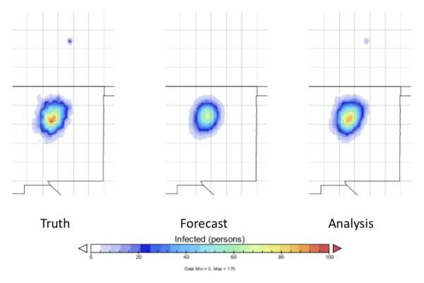
The epidemic at time 20, as shown by the spatial distribution of infectious people. A new focus of infection has appeared in Denver (the small blue spot to the north), and has been successfully assimilated. Left panel: ground truth. Center panel: forecast. Right panel: analysis.
Figure 4 (time 30) shows the epidemic gaining size, and beginning a major expansion within both Albuquerque and Denver. Every time new observations are available and are assimilated there is an improvement of the prediction of the number of infectious.
Figure 4.
The epidemic at time 30, as shown by the spatial distribution of infectious people. The infectious zone is expanding rapidly. Left panel: ground truth. Center panel: forecast. Right panel: analysis.
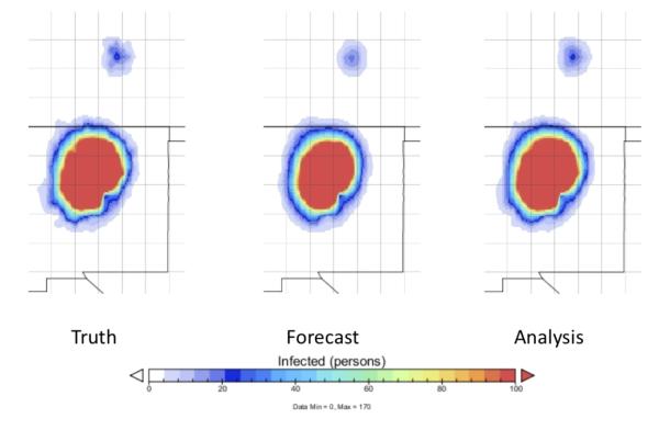
Figure 5 (time 50) shows the epidemic gaining definition within the most heavily populated urban regions. The analysis steps, after data assimilation, are now tracking the epidemic quite well.
Figure 5.

The epidemic at time 50, as shown by the spatial distribution of infectious people. Both the forecast and analysis estimates now accurately reflect the true spatial distribution of the epidemic prevalence. Left panel: ground truth. Center panel: forecast. Right panel: analysis.
We observe that the prediction improves as data is assimilated over time. The analysis thus provides a realization conditioned on all prior data and newly arrived data.
For comparison, Figure 6 shows the EnKF analysis steps at times 20 and 30, after data assimilation. Two aspects of these maps should be noted. First, the EnKF incorrectly forecasted a ring of small secondary infection loci around the primary infection locus. These loci were not in the simulation, yet they persist and even grow larger in the EnKF tracking solution. Second, the EnKF entirely missed the secondary infection in Denver, Colorado (in the north). By contrast, the EnOSI found and correctly tracked the secondary infection in Denver, and did not produce any spurious secondary infections.
Figure 6.

The epidemic at times 20 and 30 using EnKF, as shown by the spatial distribution of infectious people. Both EnKF analysis estimates display multiple spurious secondary infections, and neither displays the actual secondary infection in Denver, Colorado. Left panel: Time 20 analysis. Right panel: Time 30 analysis.
Table 1 provides the root-mean-squared error (RMSE) values for EnKF and EnOSI calculated from the current model error for each cell at the time new data arrive, both before and after assimilation. The EnOSI has a lower RMSE value than EnKF at all time steps.
Table 1.
Root mean square error (RMSE) values for EnKF and EnOSI.
| 10 | 20 | 30 | 40 | 50 | |
|---|---|---|---|---|---|
| EnKF | 0.7444 | 1.9515 | 5.7406 | 17.3312 | 41.1058 |
| EnOSI | 0.3110 | 0.9464 | 1.1430 | 2.2182 | 5.5226 |
5. Conclusion
The spread of newly emerging infectious diseases poses a serious challenge to public health in every country of the world. Tracking the spread of an epidemic in real-time can help public health officials to plan their emergency response and health care. The purpose of this paper has been to present some preliminary comparative results on the statistical tracking of emerging epidemics of infectious diseases using two Bayesian data assimilation techniques, namely ensemble Kalman filter (EnKF) and ensemble optimal statistical interpolation (EnOSI). Our simulation results suggest that EnOSI can be used to track the spatio-temporal patterns of emerging epidemics from noisy data. We found that EnOSI can efficiently adjust its estimated spatial distribution of the number of infectious, if and when the epidemic jumps from city to city. The EnOSI appears to be superior to the EnKF in two ways: it does not spuriously forecast multiple secondary outbreaks —a problem that is common to the EnKF when applied to epidemic data —and it does not require advance knowledge of the location of any secondary outbreak. The tracking accuracy in our simulations provides visual evidence of the good performance of the EnOSI approach.
The EnOSI as presented here requires the use and inversion of the state covariance matrix, which can become astronomical in size if stored as a full matrix —a grid of n × m points for a model with v state variables requires the storage of O(v2n2m2) numbers. Sparsification of the covariance matrix can decrease the computational cost somewhat, depending on the spatial assumptions used. For a completely different approach, we plan to investigate another version of OSI by Mandel (2010), which reduces the storage required by trimming the Fast Fourier Transform (FFT) of the covariance matrix, a technique also used in the FFT EnKF (Mandel et al., 2010a,b,c). We are currently developing a scheme for modeling the cross-covariance matrix for the ensemble based data assimilation methods. We hope to extend these to more general compartmental models of epidemiology.
The research reported here lays the groundwork for further efforts to investigate the utility of data assimilation for tracking diseases in real-time, and to find the best-performing algorithms for this task. Our future work includes determining the asymptotics of the EnOSI, improving the underlying spatial epidemic model, and extending our R tools for comparing other stochastic and deterministic variants of the EnKF (Anderson, 2001; Tippett et al., 2003; Beezley and Mandel, 2008; Mandel et al., 2009; Ott et al., 2004; Hunt et al., 2007). These variants aim to enhance the performance of the ensemble filters by representing the underlying model error statistics in an efficient manner. Finally, methods for incorporating long-distance human movements to track the rapid geographical spread of infectious diseases have been proposed in the literature (Brockmann, 2009; Belik et al., 2009; Merler and Ajelli, 2010; Balcan et al., 2010; Belik et al., 2010). The approach demonstrated here has not been evaluated on real data. Hence the credibility of the approach remains to be assessed. In the future, we plan to explore such spatially extended epidemic models to track emerging epidemics.
Highlights.
Ensemble optimal statistical interpolation (EnOSI) was tested as a technique for tracking spatial epidemics in real-time.
A spatial S-I-R epidemic model of an infectious disease was used to generate dynamic epidemic data for this test.
The tracking results were compared to the ensemble Kalman filter (EnKF). The EnOSI is simpler and faster in execution speed
Both the EnOSI and EnKF performed well on the main body of the epidemic, but the EnKF also forecast spurious infections.
The EnOSI successfully detected and tracked a far-flung secondary outbreak, while the EnKF missed the secondary outbreak.
Figure 1.

The initial spatial distribution of the susceptible population. The focus area of the simulation includes all of New Mexico and Colorado, and small sections of surrounding states and provinces.
Acknowledgements
This work was partially supported by Mount Royal University’s Faculty of Science and Technology Dean’s Professional Development Fund and Internal Research Grant Fund, US NIH grant 1 RC1 LM01641-01, and US NSF grants CNS-0719641, ATM-0835579, and DMS-1216481.
Footnotes
Publisher's Disclaimer: This is a PDF file of an unedited manuscript that has been accepted for publication. As a service to our customers we are providing this early version of the manuscript. The manuscript will undergo copyediting, typesetting, and review of the resulting proof before it is published in its final citable form. Please note that during the production process errors may be discovered which could affect the content, and all legal disclaimers that apply to the journal pertain.
Contributor Information
Loren Cobb, Department of Mathematical and Statistical Sciences, University of Colorado Denver Campus Box 170, PO Box 173364, Denver, CO 80217-3364, USA.
Ashok Krishnamurthy, Department of Mathematics, Physics and Engineering, Mount Royal University, Calgary, Alberta, Canada T3E 6K6.
Jan Mandel, Department of Mathematical and Statistical Sciences, University of Colorado Denver Campus Box 170, PO Box 173364, Denver, CO 80217-3364, USA.
Jonathan D. Beezley, CERFACS, 42 Avenue Gaspard Coriolis, 31057 Toulouse Cedex 1, France.
References
- Anderson JL. An ensemble adjustment Kalman filter for data assimilation. Monthly Weather Review. 2001;129:2884–903. [Google Scholar]
- Angulo JM, Yu HL, Langousis A, Madrid AE, Christakos G. Modeling of space–time infectious disease spread under conditions of uncertainty. International Journal of Geographical Information Science. 2012;26(10):1751–72. [Google Scholar]
- Bailey NTJ. Mathematical Theory of Epidemics. Griffin; 1957. [Google Scholar]
- Bailey NTJ. The Simulation of Stochastic Epidemics in Two Dimensions. Proceedings of the Fifth Berkeley Symposium on Mathematical Statistics and Probability: Biology and Problems of Health.1967. pp. 237–57. [Google Scholar]
- Balcan D, Gonçalves B, Hu H, Ramasco JJ, Colizza V, Vespignani A. Modeling the Spatial Spread of Infectious Diseases: The Global Epidemic and Mobility Computational Model. Journal of Computational Science. 2010 doi: 10.1016/j.jocs.2010.07.002. [DOI] [PMC free article] [PubMed] [Google Scholar]
- Beezley JD, Mandel J. Morphing ensemble Kalman filters. Tellus A. 2008;60(1):131–40. [Google Scholar]
- Belik V, Geisel T, Brockmann D. The impact of human mobility on spatial disease dynamics. Proceedings of the 2009 International Conference on Computational Science and Engineering-Volume 04; IEEE Computer Society; 2009. pp. 932–5. [Google Scholar]
- Belik V, Geisel T, Brockmann D. Human movements and the spread of infectious diseases. NetMob 2010: Workshop on the Analysis of Mobile Phone Networks. 2010:44–8. [Google Scholar]
- Bettencourt LMA, Ribeiro RM. Real time bayesian estimation of the epidemic potential of emerging infectious diseases. PLoS One. 2008;3(5):1–9. doi: 10.1371/journal.pone.0002185. [DOI] [PMC free article] [PubMed] [Google Scholar]
- Bettencourt LMA, Ribeiro RM, Chowell G, Lant T, Castillo-Chavez C. Intelligence and Security Informatics: Biosurveillance. ume 4506 of Lecture Notes in Computer Science. Springer; 2007. Towards real time epidemiology: data assimilation, modeling and anomaly detection of health surveillance data streams; pp. 79–90. [Google Scholar]
- Borovikov A, Rienecker M, Keppenne C, Johnson G. Multivariate error covariance estimates by Monte Carlo simulation for assimilation studies in the Pacific Ocean. Monthly Weather Review. 2005;133:2310–34. [Google Scholar]
- Brockmann D. Human Mobility and Spatial Disease Dynamics. Wiley-VCH; pp. 1–24. [Google Scholar]
- Burgers G, van Leeuwen PJ, Evensen G. Analysis scheme in the ensemble Kalman filter. Monthly Weather Review. 1998;126:1719–24. [Google Scholar]
- Castillo-Chávez C, Blower S. Mathematical Approaches for Emerging and Reemerging Infectious Diseases: An Introduction. Springer Verlag; 2002a. [Google Scholar]
- Castillo-Chávez C, Blower S. Mathematical Approaches for Emerging and Reemerging Infectious Diseases: Models, Methods and Theory. Springer Verlag; 2002b. [Google Scholar]
- Cazelles B, Chau NP. Using the Kalman filter and dynamic models to assess the changing HIV/AIDS epidemic. Mathematical Biosciences. 1997;140(2):131–54. doi: 10.1016/s0025-5564(96)00155-1. [DOI] [PubMed] [Google Scholar]
- CIESIN . Country-level population and downscaled projections based on the b2 scenario, 1990-2100. center for international earth science information network; columbia university: 2002. http://www.ciesin.columbia.edu/datasets/downscaled. Visited February 2014. [Google Scholar]
- Costa P, Dunyak J, Mohtashemi M. SoutheastCon. IEEE; 2005. Models, prediction, and estimation of outbreaks of infectious disease; pp. 174–8. Proceedings. IEEE. 2005. [Google Scholar]
- Diekmann O, Heesterbeek J. Model Building, Analysis and Interpretation. Wiley; 2000. Mathematical Epidemiology of Infectious Diseases. [Google Scholar]
- Dukic VM, Lopes HF, Polson N. Tracking flu epidemics using Google flu trends and particle learning. SSRN eLibrary. 2009 Visited February 2014. [Google Scholar]
- Eliassen A. Provisional report on calculation of spatial covariance and autocorrelation of the pressure field. In: Bengtsson L, Ghil M, Kallen E, editors. Rept. No. 5, Institute of Weather and Climate Research. Academy of Sciences; Springer-Verlag; Oslo: 1954. 1981. pp. 319–330. Reprinted in Dynamic Meteorology: Data Assimilation Methods. [Google Scholar]
- Evensen G. Using the extended Kalman filter with a multilayer quasi-geostrophic ocean model. J Geophys Res. 1992;97:17905–24. [Google Scholar]
- Evensen G. Sequential data assimilation with a nonlinear quasi-geostrophic model using Monte Carlo methods to forecast error statistics. J Geophys Res. 1994;99(C5):10143–62. [Google Scholar]
- Evensen G. Data assimilation: The ensemble Kalman filter. Springer Verlag; 2009. [Google Scholar]
- Gandin LS. Objective analysis of meteorological fields. English translation from the Russian by Israel Program for Scientific Translations. 1965 [Google Scholar]
- Gillijns S, Barrero Mendoza O, Chandrasekar J, De Moor B, Bernstein D, Ridley A. What Is the Ensemble Kalman Filter and How Well Does it Work?. Proc. of the 2006 American Control Conference (ACC2006).2006. pp. 4448–53. [Google Scholar]
- Gordon NJ, Salmond DJ, Smith AFM. Novel approach to nonlinear/non-Gaussian Bayesian state estimation. IEE Proceedings.1993. pp. 107–13. [Google Scholar]
- Hoppensteadt F. CBMS-NSF Regional Conference Series in Applied Mathematics. SIAM; 1975. Mathematical Theories of Populations, Demographics, and Epidemics. [Google Scholar]
- Houtekamer PL, Mitchell HL. Data assimilation using an ensemble Kalman filter technique. Monthly Weather Review. 1998;126(3):796–811. [Google Scholar]
- Hunt BR, Kostelich EJ, Szunyogh I. Efficient data assimilation for spatiotemporal chaos: A local ensemble transform Kalman filter. Physica D: Nonlinear Phenomena. 2007;230(1-2):112–26. [Google Scholar]
- Jégat C, Carrat F, Lajaunie C, Wackernagel H. Early detection and assessment of epidemics by particle filtering. GeoENV VI-Geostatistics for Environmental Applications: Proceedings of the Sixth European Conference on Geostatistics for Environmental Applications; Springer Verlag; 2008. pp. 23–35. [Google Scholar]
- Julier SJ, Uhlmann JK, Durrant-Whyte HF. A new approach for filtering nonlinear systems. Proc. American Control Conf..1995. pp. 1628–32. [Google Scholar]
- Kalivianakis M, Mous SLJ, Grasman J. Reconstruction of the seasonally varying contact rate for measles. Mathematical biosciences. 1994;124(2):225–34. doi: 10.1016/0025-5564(94)90044-2. [DOI] [PubMed] [Google Scholar]
- Kalman R, Bucy R. New results in linear prediction and filtering theory. Journal of Basic Engineering. 1961;83(3):95–108. [Google Scholar]
- Kalman RE. A new approach to linear filtering and prediction problems. Journal of Basic Engineering. 1960;82(1):35–45. [Google Scholar]
- Kalnay E. Atmospheric modeling, data assimilation, and predictability. Cambridge Univ Pr; 2003. [Google Scholar]
- Kendall DG. Mathematical models of the spread of infection. Mathematics and Computer Science in Biology and Medicine. 1965;213 [Google Scholar]
- Kermack WO, McKendrick AG. A contribution to the mathematical theory of epidemics. Royal Society of London Proceedings Series A. 1927;115:700–21. [Google Scholar]
- Ma S, Xia Y. Mathematical Understanding of Infectious Disease Dynamics. World Scientific; 2009. [Google Scholar]
- Mandel J. A Brief Tutorial on the Ensemble Kalman Filter. CCM UCD Report. 2007;242 http://ccm.ucdenver.edu/reports. [Google Scholar]
- Osimorph Mandel J. 2010 http://ccm.ucdenver.edu/wiki/Osimorph. Visited February 2014.
- Mandel J, Beezley JD, Cobb L, Krishnamurthy A. Data driven computing by the morphing fast Fourier transform ensemble Kalman filter in epidemic spread simulations. Procedia Computer Science. 2010a;1(1):1215–23. doi: 10.1016/j.procs.2010.04.136. ICCS 2010. [DOI] [PMC free article] [PubMed] [Google Scholar]
- Mandel J, Beezley JD, Coen JL, Kim M. Data Assimilation for Wildland Fires: Ensemble Kalman filters in coupled atmosphere-surface models. IEEE Control Systems Magazine. 2009;29(3):47–65. [Google Scholar]
- Mandel J, Beezley JD, Eben K, Jurus P, Kondratenko VY, Resler J. Data assimilation by morphing fast Fourier transform ensemble Kalman filter for precipitation forecasts using radar images. CCM UCD Report. 2010b;289 http://ccm.ucdenver.edu/reports. [Google Scholar]
- Mandel J, Beezley JD, Kondratenko VY. Gil-Lafuente AM, JMM, editors. Fast Fourier transform ensemble Kalman filter with application to a coupled atmosphere-wildland fire model. Computational Intelligence in Business and Economics, Proceedings of MS10. World Scientific. 2010c:777–84. Also available as preprint arXiv:1001.1588. [Google Scholar]
- Mandel J, Cobb L, Beezley J. On the convergence of the ensemble Kalman filter. Applications of Mathematics. 2011;56(6):533–41. doi: 10.1007/s10492-011-0031-2. [DOI] [PMC free article] [PubMed] [Google Scholar]
- Merler S, Ajelli M. The role of population heterogeneity and human mobility in the spread of pandemic influenza. Proceedings of the Royal Society B: Biological Sciences. 2010;277(1681):557–65. doi: 10.1098/rspb.2009.1605. [DOI] [PMC free article] [PubMed] [Google Scholar]
- Ott E, Hunt B, Szunyogh I, Zimin A, Kostelich E, Corazza M, Kalnay E, Patil D, Yorke J. A local ensemble Kalman filter for atmospheric data assimilation. Tellus A. 2004;56(5):415–28. [Google Scholar]
- Pierce DW. Interface to Unidata NetCDF data files package ncdf. 2010.
- R Development Core Team . R: A Language and Environment for Statistical Computing. R Foundation for Statistical Computing; Vienna, Austria: 2010. [Google Scholar]
- Rhodes CJ, Hollingsworth TD. Variational data assimilation with epidemic models. Journal of Theoretical Biology. 2009;258(4):591–602. doi: 10.1016/j.jtbi.2009.02.017. [DOI] [PubMed] [Google Scholar]
- Schmunk R. NASA Panoply NetCDF Viewer. 2013 http://www.giss.nasa.gov/tools/panoply/ Visited February 2014.
- Shaman J, Karspeck A, Yang W, Tamerius J, Lipsitch M. Real-time influenza forecasts during the 2012–2013 season. Nature communications. 2013;4 doi: 10.1038/ncomms3837. [DOI] [PMC free article] [PubMed] [Google Scholar]
- Talagrand O. Bayesian estimation. Optimal interpolation. Statistical linear estimation. In: Swinbank R, Shutaev VP, Lahoz WA, editors. Data assimilation for the Earth system. Springer; Netherlands: 2003. pp. 21–35. [Google Scholar]
- Tippett MK, Anderson JL, Bishop CH, Hamill TM, Whitaker JS. Ensemble square root filters. Monthly Weather Review. 2003;131:1485–90. [Google Scholar]