

Abstract
In disease screening, the combination of multiple biomarkers often substantially improves the diagnostic accuracy over a single marker. This is particularly true for longitudinal biomarkers where individual trajectory may improve the diagnosis. We propose a pattern mixture model (PMM) framework to predict a binary disease status from a longitudinal sequence of biomarkers. The marker distribution given the disease status is estimated from a linear mixed effects model. A likelihood ratio statistic is computed as the combination rule, which is optimal in the sense of the maximum receiver operating characteristic (ROC) curve under the correctly specified mixed effects model. The individual disease risk score is then estimated by Bayes’ theorem, and we derive the analytical form of the 95% confidence interval. We show that this PMM is an approximation to the shared random effects (SRE) model proposed by Albert (2012. A linear mixed model for predicting a binary event from longitudinal data under random effects mis-specification. Statistics in Medicine 31(2), 143–154). Further, with extensive simulation studies, we found that the PMM is more robust than the SRE model under wide classes of models. This new PPM approach for combining biomarkers is motivated by and applied to a fetal growth study, where the interest is in predicting macrosomia using longitudinal ultrasound measurements.
Keywords: Area under ROC curve, Fetal growth, Longitudinal biomarker combination, Macrosomia, Pattern mixture model, Risk estimation
1. Introduction
It is a common practice that multiple diagnostic tests or biomarkers are used to screen for disease. Any one of the biomarkers alone may not have high classification accuracy; however, combining multiple markers often improves the accuracy substantially. The combined biomarker may guide the physician's decision on disease diagnosis, treatment, or prevention strategies. From a patient's perspective, on the other hand, one may be more interested to know his her own disease risk given the observed markers. Therefore, both disease classification and risk prediction are of interest.
Biomarker combination methods in cross-sectional studies have been widely discussed in the literature. Su and Liu (1993) showed that the linear discriminant function gives the best linear combination under a normal distribution assumption. Liu and others (2005) extended their work by considering maximizing sensitivity over a partial range of specificity. Pepe and Thompson (2000) first proposed a distribution-free approach to estimating the best linear combination that maximizes the empirical area under the receiver operating characteristic (ROC) curve (AUC). McIntosh and Pepe (2002) showed that the risk score, defined as the disease probability given the observed biomarkers, is the optimal combination of biomarkers. Pepe and others (2006) compared the approaches of maximizing the logistic likelihood versus maximizing AUC, and found that the latter is more robust to an incorrect risk model. Ma and Huang (2007), who extended the results of Pepe and Thompson (2000), maximized a sigmoid AUC estimator that approximates the true AUC, and derived the asymptotic properties of the combination rule. Liu and others (2011) considered a non-linear combination of repeatedly measured biomarkers that only used the minimum and maximum marker values. Lin and others (2011) discussed the selection and combination of biomarkers with a lasso-type  penalty term. Little attention has been paid to the combination of longitudinal biomarkers.
When one or multiple markers are measured repeatedly over time, the disease diagnosis should take into account their trajectory and correlation structures. Recently, Albert (2012) proposed a shared random effects (SRE) model to evaluate the predictive accuracy of longitudinal biomarkers. Under a Gaussian random effects assumption, his approach simplifies to a two-step procedure. In the first step, a linear mixed model is fit to the longitudinal markers. In the second step, a binary regression is fit to the disease outcome, using the predicted random effects as covariates. Regression calibration techniques are used to account for the fact that the random effects are estimated with uncertainty. Albert (2012) showed that the two-step procedure is easy to implement, and behaves well when the Gaussian random effects assumption fails to hold.
In this paper, we develop an alternative method for the longitudinal biomarker combination. For simplicity of presentation, we focus on the situation of one longitudinal biomarker, and demonstrate the straightforward extension to multiple sequences of biomarkers in supplementary material available at Biostatistics online. A pattern mixture model (PMM) framework is adopted that models the marker distribution for the cases and controls separately. We then estimate the joint density function of the marker given the disease status, and hence construct the likelihood ratio statistic as the combination rule. The individual disease risk can be estimated as a byproduct, and we derive the analytical form of the 95% confidence interval (CI) for the estimated risk. We explore the difference between the SRE and PMM methods both theoretically and with simulation studies, and consequently make recommendations for their practical use. Fieuws and others (2008) considered the PMM framework to predict survival outcomes with longitudinal biomarkers. Their focus was on estimating the survival function, while we are interested in evaluating the classification accuracy and estimating the disease risk.
This paper is motivated by a data set from the Scandinavian infant growth project, a large fetal growth study conducted in the early 1990s (Bakketeig and others, 1993). Longitudinal ultrasound measurements are collected at approximately 17, 25, 33, and 37 weeks of gestation, and the interest is in predicting macrosomia (defined by a birth weight larger than 4000 g) with the longitudinal observations. We compare the performance of PMM and SRE estimators using this data set.
In Sections 2.1 and 2.2, we briefly review the SRE estimator and propose the new PMM approach to estimate the combined marker. In Section 2.3, we make theoretical comparisons between SRE and PMM methods. Section 3 discusses the covariate adjustment with the PMM approach and proposes the covariate-dependent combination rule. Section 4 presents extensive simulation studies that examine the performance of the proposed PMM estimator, followed by the analysis of the fetal growth data in Section 5. We conclude in Section 6 with a discussion.
2. Methods
Let  be the binary indicator of the
  th subject being diseased (
 ) or healthy (
 ) for
) for  . Without loss of generality, assume that the first
  subjects are diseased and the last
  subjects are healthy. Let
  be the univariate longitudinal biomarker with observations taken at times
  . We suppress the subscript
  when there is no confusion. For the fetal growth application,
  represents the occurrence of macrosomia and
  reflects longitudinal ultrasound measurements at different gestational ages.
2.1. SRE approach
SRE models are commonly used when two dependent processes need to be modeled simultaneously, e.g. in the context of missing data (Wu and Carroll, 1988). Albert (2012) first adopted the SRE approach to solve the biomarker combination problem. He proposed a linear mixed model given by
 |
(2.1) |
where  and
and  are the design matrices of the fixed and random effects,
  is the vector of fixed effects parameters,
  is the vector of random effects, and
  is the vector of residuals. Then the binary random variable
  can be linked to the longitudinal process as
 |
(2.2) |
where  is the vector of subject-specific covariates,
  is a known function of the random effects, and
  characterizes the strength of association between the longitudinal process and the binary outcome. Motivated by the fetal growth example, Albert (2012) used a quadratic growth curve for both the fixed and random effects in (2.1):
 |
where  denotes the gestational age of the
  th fetus at the
  th visit. In the binary outcome model (2.2),
  is taken to be
  , representing the projected deviation from an average fetus at time
  , where
  is a time point near birth, e.g. 39 weeks.
To estimate the SRE (2.1) and (2.2), one may integrate out the random effects and maximize the likelihood constructed by the joint density of  and
and  . Albert (2012) noted that the parameter estimation can be greatly simplified if the random effects are normally distributed with a probit link function. The likelihood function can be written in the form of
  , where
  and
and  . Now
. Now  only involves the parameters of the fixed effects and variance components in (2.1), and the latter is shown to have an explicit expression that only includes the parameters
  and
and  in (2.2):
 |
where  . A simple choice of the
  function could be a linear combination of the random effects. This suggests a two-step estimating procedure: the first step involves maximizing
  by fitting a linear mixed effects model; the second step fits a binary regression of
  versus the empirical Bayes predictor,
  , and a regression calibration approach is used to account for the estimation variability of
  .
.
The SRE makes a strong assumption on how the individual random effects influence the disease risk, which is not easy to verify. Although it is robust to the random effects distribution, it may not be robust to the mis-specified link function. If the probit link is incorrect, the risk prediction could be biased. Therefore, we propose an alternative PMM framework that relaxes the binary regression assumption (2.2).
2.2. PMM approach
We directly makes the assumption of a linear mixed model on  , with the outcome model stratified by disease status. The index
  can be reorganized such that the first
  subjects are diseased and the last
  are healthy. Let
  be the set of subscripts for the subjects with
  .
.
 |
(2.3) |
 |
(2.4) |
where  are the vectors of fixed effects,
  are the vectors of random effects,
  and
and  are their design matrices, and
  are the vectors of random errors for
  . Assume that
  and
and  independently follow multivariate normal distributions:
 |
where  and
and  are the variance components. In this subsection, we temporarily assume that the design matrices
  and
and  are expanded by the observation times
  only, and no covariates are observed. In Section 3, we will discuss the extension that allows for individual covariates. We can now write
 |
(2.5) |
where  and
and  for
for  .
.
Disease classification can be regarded as analogous to a hypothesis testing problem. Let  be a combination rule that maps the
  -dimensional longitudinal marker
  to a univariate marker
  . Without loss of generality, suppose that a larger value of
  is more indicative of disease. The sensitivity (Se) and 1
 specificity (
 ) at a cutoff point
  are given by
 |
They are analogous to the power and type I error of the statistic  if we view
  as the null hypothesis and
  as the alternative hypothesis. We note that the null and alternative hypothesis should be written in terms of an unknown parameter instead of a random variable
  , but here we allow the slightly abused notation just for illustrative purposes. Using the same argument as the Neyman–Pearson Lemma, it follows that the likelihood ratio
 |
is the most “powerful” test. Translating to the ROC curve context, it suggests that the sensitivity of  is uniformly greater than any other function
  at any specificity level, and hence
  is the optimal combination rule in terms of the diagnostic accuracy. This result was also recognized by McIntosh and Pepe (2002). For this classification problem, the likelihood ratio statistic is used to establish a combination rule for the longitudinal biomarkers, and hence calculate the individual disease risk score. It is different from the traditional hypothesis testing framework in that we are not interested in the distribution of the test statistics, but rather in the optimal classification ability of the statistic, represented by the ROC curve or its area.
Under the PMM setting,  is readily available as
 |
(2.6) |
which is a quadratic function of  , and degenerate to a linear function if
  . Furthermore, the disease risk score,
  , can be expressed as a function of
  using Bayes’ theorem:
 |
(2.7) |
Therefore, the risk score is simply a byproduct of the likelihood ratio combination computation. For a fixed observation of the marker value  , let
, let  and let
  be the estimated version of
  with the unknown parameters
  ,
,  , and
, and  all replaced by their maximum likelihood estimates. The following theorem gives the asymptotic distribution of
  .
.
Theorem 2.1 —
If the PMM model assumption given by (2.3) and (2.4) is true, as
,
The proof of the above theorem, as well as the explicit formula for  , is given in supplementary material available at Biostatistics online.
2.3. Comparison of SRE and PMM
In the missing data literature, the SRE models could be approximated by PMMs (Wu and Carroll, 1988; Wu and Bailey, 1989). Here we make a similar argument: if the data are indeed generated from an SRE model, the PMM framework would lead to nearly correct inference.
Suppose that the true model is given by (2.1) and (2.2). Then
 |
The second equality follows from the true model (2.1). Now, if we approximate  by a multivariate normal distribution, then
  becomes a linear mixed model. This suggests that the PMM is an approximation of the SRE; that is, if the SRE is the correct model, the PMM will perform well.
Conversely, if the data are actually generated by the PMM (2.3) and (2.4), the SRE model assumption could be seriously biased. To illustrate this, we consider a simple model:
 |
where the cases and controls have different intercepts and slopes over time  , but the same variance components. In other words,
  and
and  both follow multivariate normal distributions with the same variance matrix
  . The likelihood ratio combination can be derived as
 |
(2.8) |
where  is the
  matrix of ones and
  is the
  identity matrix. If we instead fit a marginal model for
  regardless of
  , then we have
 |
where  ,
,  and
and  . Now
. Now  is a finite mixture of normal distributions whose variance is
  . The best linear unbiased predictor
  serves as the combined marker:
 |
Note that  is a compound symmetry matrix, so that the combination of
  is proportional to the arithmetic average
  . But the optimal combination (2.8) assigns different weights on
  if
if  . That is, the SRE model and the PMM are equivalent only when the effect of
  is the same for every
  .
.
There are two advantages of our proposed method compared with the SRE model in Albert (2012). First, when the PMM is correct, the Neyman–Pearson Lemma guarantees that the likelihood ratio statistic is the optimal combination in terms of maximizing AUC. When the SRE model is correct, the PMM can still closely approximate the underlying data distribution. So, in a sense, the PMM is more robust than SRE. Second, the computation of the PMM is relatively simple with standard software, even if the longitudinal design is unbalanced, or the random effects distribution is assumed to be non-Gaussian. As a comparison, Albert (2012) relies on the probit link function of the binary regression. If other link functions are used, the regression calibration technique does not work any more, and the maximization of the marginal likelihood could be more time-consuming.
3. Extension to covariate-specific combination
In many longitudinal studies, individual covariates are also observed and may be helpful in predicting the disease. For example, mother's age and body mass index (BMI) may play an important role in the prediction of macrosomia. When covariates affect the magnitude and or accuracy of a marker, it is recommended that they should be adjusted in the ROC analysis (Zhou and others, 2002; Pepe, 2003), and so should they in the biomarker combination (Liu and Zhou, 2013). Denote
  to be the vector of covariates of the
  th subject. The pattern mixture distributions, given by (2.5) without covariates, need to be modified by conditioning on
  :
:
 |
where  and
and  . It should be noted that the design matrices
  and
and  are expanded by
  and observations times
  , so the covariates affect both the conditional mean and variance of
  . Applying the Neyman–Pearson Lemma on the subpopulation stratified by
  , the covariate-dependent combination rule
 |
is optimal in terms of the covariate-specific ROC curve.
The disease risk score can be shown as
 |
(3.1) |
Thus, for implementation, we need to fit an additional model for  , and that could be easily done with logistic regression. This binary regression model is purely based on observed variables, so the model diagnostics are much easier than the binary regression in SRE, where the regressors include latent variables.
4. Simulation studies
4.1. Simulation one
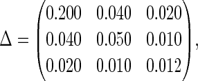
In the first simulation study, we compared the performance of the proposed PMM approach with the SRE models in Albert (2012) under various settings of correct or mis-specified models. Consider one biomarker with  observations at times
  . If the true model is SRE, the marker distribution was generated from the following linear mixed effects model:
 |
(4.1) |
where 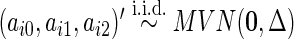 and
and 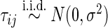 . We set
 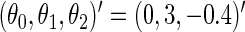 ,
,  , and
, and
 |
with a correlation of 0.4 among the random effects. The disease model is given by
 |
(4.2) |
where we took  ,
,  and varied
  (or
(or  ) to reflect high (low) disease prevalence (about 50% and 20%, respectively). This setting is referred to as Scenario A0. The setup of the linear combination
  resembles that of Albert (2012), which implies that the extrapolated individual random effects at a future time
  is related to the binary outcome. For predicting macrosomia using longitudinal ultrasound data,
  is chosen as a time near birth, e.g. 39 weeks.
If the true model is the PMM, we first generated  from
from  with
with  or
or  . Then the longitudinal marker for the cases and controls were generated from
 |
(4.3) |
where  and
and  . The parameter values were taken to be
  ,
,  ,
,  ,
,  ,
,  , and
, and  . This setting is referred to as Scenario B0. We fixed the sample size to be 2000. The first half were the training sample for estimating the combination rule; the remaining half were the test sample to evaluate the prediction accuracy. The results of 500 simulations are shown in Table 1. We reported the AUC for the combination rule, and the mean squared error (MSE) of the predicted disease risk. Under Scenario A0, the PMM and SRE combination rules yield very close AUC and MSE. But under B0, SRE does not approximate the PMM very well, and the diagnostic performance of the PMM is better than SRE.
Table 1.
Simulation results for correctly specified SRE (A0) and PMM (B0) models
 |
True AUC | Method | AUC ( ) ) |
MSE ( ) ) |
|
|---|---|---|---|---|---|
| A0 | High | 0.866 | SRE | 0.854 (1.13) | 0.156 (0.62) |
| PMM | 0.852 (1.14) | 0.157 (0.62) | |||
| Low | 0.884 | SRE | 0.872 (1.30) | 0.108 (0.64) | |
| PMM | 0.869 (1.29) | 0.109 (0.62) | |||
| B0 | High | 0.769 | SRE | 0.743 (1.53) | 0.205 (0.54) |
| PMM | 0.765 (1.50) | 0.193 (0.58) | |||
| Low | 0.769 | SRE | 0.743 (2.08) | 0.132 (0.68) | |
| PMM | 0.762 (2.00) | 0.124 (0.71) |
We also conducted simulation studies with model mis-specification under the SRE and the PMM framework (Scenarios A1–A8 and B1–B5, respectively). The detailed settings are described in supplementary material available at Biostatistics online. Similarly to the simulation settings in Albert (2012), we examined the mis-specified random effects distributions under the SRE model (A3–A5), and found that AUC and MSE are both quite robust to this mis-specification. We have similar findings for the mis-specified error distribution (A1–A2) and link function (A6–A8) as well; all the estimated AUC are close to the truth. We note that with the mis-specified models, the PMM still closely approximates the SRE model, but the converse is not true. With a mis-specified error distribution under the PMM (B1–B2), the estimated AUC using the PMM method is close to the truth, but the SRE method does not perform as well. Under two-component mixture normal random effects, the performance of the PMM is good when the two normals in the mixture are relatively close (B3), but becomes worse as the two normals get more separated (B4–B5). In this case, we could consider finite mixture Gaussian random effects models under the PMM framework (Proust and Jacqmin-Gadda, 2005).
4.2. Simulation two
In this simulation study, we examine the performance for estimating individualized risks and their associated CIs. We adopt the settings in Scenario A0 and B0, but fix a small test sample of 100 subjects for all the 500 simulations. The training sample consists of 1000 subjects as before. For the SRE method, we perform 200 bootstrap resampling to obtain the 95% CI for the estimated disease risk. For the PMM method, we calculate both the bootstrap and analytical 95% CI as given in Theorem 2.1. The average estimated disease risks as well as the 95% CI coverage are displayed in Figure 1. When the SRE model is correct (A0), the SRE method is consistent with close-to-nominal CI coverage. The PMM method works well for the majority of the test samples, and fails only when the disease risk is extremely small or large. On the other hand, when the PMM model is correct (B0), the performance of the SRE method is unsatisfactory with large bias and poor CI coverage. The PMM disease risk is consistently estimated for every subject in the test sample.
Fig. 1.

Simulation results of the estimated disease risk for 100 out-sample subjects under the SRE (A0) and PMM (B0) models: (a) estimated versus true disease risk in Scenario A0; (b) 95% CI coverage rate in Scenario A0; (c) estimated versus true disease risk in Scenario B0; (d) 95% CI coverage rate in Scenario B0.
From the above two simulation studies, we would recommend the PMM method in general because of its robustness to model mis-specifications. The SRE method is appropriate only if one is certain about the SRE structure of (2.1) and (2.2).
5. Example: fetal growth data
Our analysis sample consists of  subjects. The longitudinal marker is the mean abdominal diameter in log scale, taken at 17, 25, 33, and 37 weeks of gestation. A more detailed description of the study can be found in Bakketeig and others (1993). We fit the same models as in the simulation studies: the fixed effects and random effects both include the linear and quadratic terms of time
  . The quadratic model was found to provide a good fit to the fetal growth data (Albert, 2012). That said, both the PMM and SRE approaches could easily incorporate a spline formulation for the mean structure. We randomly selected 600 subjects as the training sample and the remaining 516 subjects serve as the test sample.
For illustrative purposes, our main analysis ignores all the subject covariates. The fitted parameters are shown in Table 2. The stratified mean of  for the cases and controls are estimated to be
  and
and  using the PMM method. The means of the cases are greater than the controls, although the difference is not large. As we will see later, the overall prediction accuracy is still satisfactory, because the variability at each time point is relatively small and the within-subject correlation is relative large. The marginal mean given by the SRE method is
  , which lies in between
  and
and  . The SRE method estimates
  to be
to be
 |
and the PMM method estimates  and
and  to be
to be
 |
respectively. The stratified variances are similar in the first two time points but differ in the last two for the cases and controls, indicating that the PMM combination rule may not be linear. We performed a likelihood ratio test over the whole sample for a common variance component of the random effects, and found a  -value of 0.037, justifying the use of stratified models.
Table 2.
Estimated coefficients for the SRE and PMM models in the fetal growth study
| PMM |
|||
|---|---|---|---|
| Controls | Cases | SRE | |
 |
3.6415 (0.0047) | 3.6496 (0.0102) | 3.6429 (0.0042) |
 |
0.5996 (0.0066) | 0.6142 (0.0148) | 0.6022 (0.0060) |
 |
 0.0801 (0.0021) 0.0801 (0.0021) |
 0.0780 (0.0047) 0.0780 (0.0047) |
 0.0797 (0.0019) 0.0797 (0.0019) |
 |
0.099 | 0.098 | 0.099 |
 |
0.128 | 0.133 | 0.129 |
 |
0.037 | 0.040 | 0.038 |
 |
 0.846 0.846 |
 0.851 0.851 |
 0.845 0.845 |
 |
0.734 | 0.741 | 0.735 |
 |
 0.972 0.972 |
 0.977 0.977 |
 0.972 0.972 |
 |
0.035 | 0.037 | 0.035 |
| AUC | 0.813 | 0.782 | |
We chose five subjects from the test sample, namely, “average fetus”, “large fetus”, “small fetus”, “fast grower”, and “slow grower”. The growth trajectory of the five subjects as well as the estimated disease risks are shown in Figure 2. The PMM and SRE estimation could be quite different for assessing individualized risk. As we do not know the true disease risk in the real example and the five subjects were chosen post hoc, this result cannot be over-interpreted. However, we do observe that the PMM method leads to a moderate amount of improvement in the out-sample AUC (0.813) compared with the SRE approach ( ). The plot of ROC curves were provided in supplementary material available at Biostatistics online, and we find that the ROC curve for the PMM is uniformly higher than for the SRE model. This is interpreted as, for any given decision threshold with a fixed specificity, the PMM always yields a higher sensitivity than the SRE model.
Fig. 2.

The growth trajectory of five selected subjects from the test sample, with their estimated disease risks using the PMM and SRE approaches.
In the secondary analysis, we incorporate four subject covariates into both the PMM and the SRE model: mother's age, pre-pregnancy BMI, history of small-for-gestational-age birth, and cigarettes smoked per day at enrollment. The estimated regression coefficients are reported in supplementary material available at Biostatistics online. The estimated AUC and MSE, as well as the estimated disease risks for the five example subjects are listed in Table 3. The 95% CI for PMM risk is calculated using the analytic variance formula; the 95% CI for SRE risk is calculated from 1000 bootstrap samples. The AUCs for PMM and SRE methods both improve after including the covariate information. The PMM still outperforms the SRE model with higher AUC.
Table 3.
Estimated disease risks for the five selected subjects in the test sample, and the AUC and MSE calculated in the whole test sample for the PMM and SRE estimators, with and without covariate adjustment
| Without covariates |
With covariates |
|||
|---|---|---|---|---|
| SRE | PMM | SRE | PMM | |
| Average fetus | 0.153 (0.120–0.183) | 0.179 (0.134–0.235) | 0.118 (0.066–0.170) | 0.152 (0.092–0.241) |
| Large fetus | 0.741 (0.604–0.853) | 0.381 (0.089–0.794) | 0.399 (0.141–0.650) | 0.099 (0.014–0.459) |
| Small fetus | 0.002 (0.000–0.008) | 0.002 (0.000–0.022) | 0.002 (0.000–0.010) | 0.002 (0.000–0.021) |
| Fast grower | 0.210 (0.126–0.284) | 0.468 (0.275–0.671) | 0.114 (0.021–0.271) | 0.276 (0.085–0.609) |
| Slow grower | 0.085 (0.041–0.157) | 0.002 (0.000–0.023) | 0.021 (0.002–0.071) | 0.000 (0.000–0.005) |
| AUC | 0.782 | 0.813 | 0.814 | 0.829 |
| MSE | 0.118 | 0.112 | 0.113 | 0.111 |
6. Discussion
In this paper, we proposed a PMM framework to handle the problem of prediction from longitudinal biomarkers. The marker values are fitted by linear mixed effects models for the cases and controls separately. We then derived the likelihood ratio statistic as the optimal combination rule, and the disease risk score is then estimated with the Bayes theorem. The likelihood ratio statistic determines the form of the combination rule, and often results in a non-linear combination. In theoretical derivations and simulation studies, we showed that the PMM method can closely approximate the SRE model in Albert (2012). Furthermore, our simulation studies showed that it is robust to many settings of model mis-specifications. As pointed out by an anonymous referee, the PMM method we proposed does not handle the treatment of patients during the followup period. In our application of predicting macrosomia, this is not a serious concern as no relevant treatment was involved. However, in some situations such as predicting more aggressive diseases, treatment or prevention procedures may take place right after observing changes in the biomarkers. In this case, the time-varying treatment scheme needs to be modeled together with the biomarker process, which is an area of future research.
The PMM framework was extended in several ways. First, with additional covariates information, we derived the PMM combination rule that yields optimal covariate-specific ROC curves. We found in the fetal growth example that incorporating subject covariates improved the prediction accuracy of macrosomia. Second, the extension to multivariate biomarkers is straightforward, by multivariate random effects models, as we outlined in supplementary material available at Biostatistics online. In addition, it is not difficult for the PMM to handle unbalanced longitudinal data (e.g. due to dropout), and different observation times for each subject (e.g. a subject missed a scheduled examination but made it up two weeks later).
The PMM method is generally recommended for practical use if one is interested in estimating the disease risk or making a diagnosis on patients. However, if the interest is in finding the risk factors of the disease conditioning on the markers, the SRE method is more favorable as those parameters can be directly estimated from (2.2). We can see from (3.1) that the PMM method, on the contrary, does not allow direct inference on the individual covariates, as the covariates affect the disease risk in a complicated manner.
We assumed that the biomarkers follow normal distribution after suitable transformations in the fetal growth study. There are several reasons why this assumption is not crucial in our proposed method. First, we showed in the simulation studies that when the random effects and error distributions deviate from normal, the PMM method still yields good prediction accuracy. Second, when binary or ordinal markers arise in other circumstances, such as in radiology studies, the PMM method can still be adapted to incorporate the generalized linear mixed models for the longitudinal markers. In this case, the likelihood ratio combination would involve intractable integrals that can be evaluated using numerical approaches. Another potentially interesting future work is to consider the prediction of other types of outcome events, such as longitudinal continuous, binary, and survival outcomes.
7. Software
R functions for the proposed estimators are available on request from the corresponding author.
Supplementary material
Funding
This research is supported by the Intramural Research Program of the National Institute of Health (NIH), Eunice Kennedy Shriver National Institute of Child Health and Human Development (NICHD).
Supplementary Material
Acknowledgements
This study utilized the high-performance computational capabilities of the Biowulf Linux cluster at NIH, Bethesda, MD (http://biowulf.nih.gov). The authors thank the associate editor and referees for their thoughtful comments that improved the quality of the paper. Conflict of Interest: None declared.
References
- Albert P. S. A linear mixed model for predicting a binary event from longitudinal data under random effects misspecification. Statistics in Medicine. 2012;31(2):143–154. doi: 10.1002/sim.4405. [DOI] [PMC free article] [PubMed] [Google Scholar]
- Bakketeig L. S., Jacobsen G., Hoffman H. J., Lindmark G., Bergsjø P., Molne K., Rødsten J. Pre-pregnancy risk factors of small-for-gestational age births among parous women in scandinavia. Acta Obstetricia et Gynecologica Scandinavica. 1993;72(4):273–279. doi: 10.3109/00016349309068037. [DOI] [PubMed] [Google Scholar]
- Fieuws S., Verbeke G., Maes B., Vanrenterghem Y. Predicting renal graft failure using multivariate longitudinal profiles. Biostatistics. 2008;9(3):419–431. doi: 10.1093/biostatistics/kxm041. [DOI] [PubMed] [Google Scholar]
- Lin H., Zhou L., Peng H., Zhou X. H. Selection and combination of biomarkers using ROC method for disease classification and prediction. Canadian Journal of Statistics. 2011;39(2):324–343. [Google Scholar]
- Liu C., Liu A., Halabi S. A min–max combination of biomarkers to improve diagnostic accuracy. Statistics in Medicine. 2011;30(16):2005–2014. doi: 10.1002/sim.4238. [DOI] [PMC free article] [PubMed] [Google Scholar]
- Liu A., Schisterman E. F., Zhu Y. On linear combinations of biomarkers to improve diagnostic accuracy. Statistics in Medicine. 2005;24(1):37–47. doi: 10.1002/sim.1922. [DOI] [PubMed] [Google Scholar]
- Liu D., Zhou X. H. ROC analysis in biomarker combination with covariate adjustment. Academic Radiology. 2013;20(7):874–882. doi: 10.1016/j.acra.2013.03.009. [DOI] [PMC free article] [PubMed] [Google Scholar]
- Ma S., Huang J. Combining multiple markers for classification using ROC. Biometrics. 2007;63(3):751–757. doi: 10.1111/j.1541-0420.2006.00731.x. [DOI] [PubMed] [Google Scholar]
- McIntosh M. W., Pepe M. S. Combining several screening tests: optimality of the risk score. Biometrics. 2002;58(3):657–664. doi: 10.1111/j.0006-341x.2002.00657.x. [DOI] [PubMed] [Google Scholar]
- Pepe M. S. The Statistical Evaluation of Medical Tests for Classification And Prediction. Oxford: Oxford University Press; 2003. [Google Scholar]
- Pepe M. S., Cai T., Longton G. Combining predictors for classification using the area under the receiver operating characteristic curve. Biometrics. 2006;62(1):221–229. doi: 10.1111/j.1541-0420.2005.00420.x. [DOI] [PubMed] [Google Scholar]
- Pepe M. S., Thompson M. L. Combining diagnostic test results to increase accuracy. Biostatistics. 2000;1(2):123–140. doi: 10.1093/biostatistics/1.2.123. [DOI] [PubMed] [Google Scholar]
- Proust C., Jacqmin-Gadda H. Estimation of linear mixed models with a mixture of distribution for the random effects. Computer Methods and Programs in Biomedicine. 2005;78(2):165–173. doi: 10.1016/j.cmpb.2004.12.004. [DOI] [PMC free article] [PubMed] [Google Scholar]
- Su J. Q., Liu J. S. Linear combinations of multiple diagnostic markers. Journal of the American Statistical Association. 1993;88(424):1350–1355. [Google Scholar]
- Wu M. C., Bailey K. R. Estimation and comparison of changes in the presence of informative right censoring: conditional linear model. Biometrics. 1989;45(3):939–955. [PubMed] [Google Scholar]
- Wu M. C., Carroll R. J. Estimation and comparison of changes in the presence of informative right censoring by modeling the censoring process. Biometrics. 1988;44(1):175–188. [Google Scholar]
- Zhou X. H., McClish D. K., Obuchowski N. A. Statistical Methods in Diagnostic Medicine. New York: Wiley; 2002. [Google Scholar]
Associated Data
This section collects any data citations, data availability statements, or supplementary materials included in this article.