

Abstract
Purpose
EPRI has surfaced as a promising non-invasive imaging modality that is capable of imaging tissue oxygenation. Due to extremely short spin-spin relaxation time, EPRI benefits from single point imaging and inherently suffers from limited spatial and temporal resolution, preventing localization of small hypoxic tissues and differentiation of hypoxia dynamics, making accelerated imaging a crucial issue.
Method
In this study, methods for accelerated single point imaging were developed by combining a bilateral k-space extrapolation technique with model-based reconstruction that benefits from dense sampling in the parameter domain (measurement of the T2* decay of an FID). In bilateral k-space extrapolation, more k-space samples are obtained in a sparsely sampled region by bilaterally extrapolating data from temporally neighboring k-spaces. To improve the accuracy of T2* estimation, a principal component analysis (PCA)-based method was implemented.
Result
In a computer simulation and a phantom experiment, the proposed methods showed its capability for reliable T2* estimation with high acceleration (8-fold, 15-fold, and 30-fold accelerations for 61×61×61, 95×95×95, and 127×127×127 matrix, respectively).
Conclusion
By applying bilateral k-space extrapolation and model-based reconstruction, improved scan times with higher spatial resolution can be achieved in the current SP-EPRI modality.
Keywords: EPR Imaging, Quantitative Imaging, Single Point Imaging, Model-based Reconstruction, k-Space Extrapolation
Introduction
Electron Paramagnetic Resonance Imaging (EPRI) is a non-invasive imaging technique that measures the spatial distribution of unpaired electrons, akin to protons in MRI. Owing to the recent development of biologically compatible spin probes (1-3), EPRI has emerged as a promising non-invasive imaging modality capable of dynamically and quantitatively imaging in vivo tissue oxygenation. However, due to extremely short spin-spin relaxation times, slice-selective imaging and conventional frequency encoding techniques are difficult to achieve and single-point imaging (SPI) techniques are often utilized to improve image quality (4,5). In single point EPRI (SP-EPRI), gradients remain constant during excitation, and data is acquired immediately after transmit dead time until no signal remains. Thus SP-EPRI is rich in the spectral domain, but inherently suffers from reduced spatial and temporal resolution due to the time needed for a globally phase-encoded acquisition.
SPI also exhibits a “zoom-in” effect due to the use of constant gradients, where k-space samples spread and objects enlarge (as FOV decreases) at increasing phase encoding time delays. Recently, we proposed a method based on gridding termed k-space extrapolation (KSE) to maintain FOV across all phase encoding time delays and to improve the reliability of parameter estimation (6). Although this method improves temporal resolution (by a factor of 3) by eliminating the need of multiple data acquisitions (7) required to secure multiple images with same FOV, further reduction in acquisition time is needed for SPI. In MRI, a myriad of techniques have been proposed to accelerate imaging, such as parallel imaging (8-10), partial Fourier reconstruction (11) (also applied to SP-EPRI (12)), and compressed sensing reconstruction (13). Among them, compressed sensing has recently surfaced as a promising method that can accelerate image acquisition by enabling high ratio of undersampling without a loss of image quality.
Compressed sensing was first introduced in the area of signal processing and information theory (14,15), which was based on the idea that signals can be reconstructed from highly reduced measurements if the signals show sparse representation. Recently, there have been many successful efforts employing compressed sensing to medical imaging (16-20). Since medical images usually do not show sparse representation by themselves (except some special cases such as angiography), compressed sensing applications benefit from transform domain sparsity that is achieved by transformations such as the discrete wavelet transform (DWT).
Unfortunately, the application of compressed sensing is difficult to employ in SP-EPRI due to its small matrix size that inhibits transform domain sparsity. However, since SP-EPRI acquires abundant data in the parameter domain (measurement of the T2* decay of the FID) and the T2* relaxation model is monoexponential and well-known, SP-EPRI can benefit from model-based reconstruction techniques that simultaneously use k-p-space data in reconstructing images. In such model-based methods, an overcomplete dictionary or principal component analysis (PCA) can be used to sparsify the acquired data and improve T2* estimation (19,21,22).
In this study, we improved our previous KSE technique to add parameter domain reconstruction and further enhance spatial and temporal resolution in SP-EPRI. The improved, bilateral k-space extrapolation (bi-KSE) allows more sample points to be secured in a target k-space by bilaterally extrapolating k-space samples from the neighboring k-spaces. In addition, a 3 zone sampling strategy was utilized for which a different sampling criterion was applied to each zone while taking advantage of the large degree of conjugate symmetry possible in EPRI. Model-based reconstruction using PCA (19) was implemented to further improve accuracy of T2* parameter estimation. During the reconstruction process, aliasing artifacts caused by undersampling are iteratively suppressed by promoting sparsity of PC coefficient maps in the DWT domain.
Methods
k-Space Sampling Strategy
An incoherent sampling trajectory is a necessary component for sparsity-promoting reconstruction techniques where noise-like aliasing artifacts are desirable. The trajectory used herein utilizes conjugate symmetry and randomized sampling. Owing to pure phase encoding and low B0 field (10 mT), image phase in SP-EPRI is more tractable than in MRI (12). The reconstructed images in Figure 1 show a high degree of conjugate symmetry is possible in SP-EPRI. Therefore, we exploited conjugate symmetry when prescribing randomized sampling patterns by avoiding all symmetric points. Further, we designed a hierarchical random sampling scheme to effectively maximize the number of k-space samples in an undersampled acquisition.
Figure 1.

High degrees of partial Fourier sampling with conjugate symmetry can be utilized in SP-EPRI.
Figure 2-a shows an example of the proposed hierarchical random sampling scheme, where k-space is segmented into 3 zones. Zone 1 is a fully sampled central region. Zone 2 is a region where k-space is undersampled by a factor of 2, which is converted to a fully sampled region after the application of conjugate symmetry. This large fully sampled region is required to maximize the performance of model-based reconstruction explained in later section. Zone 3 is more sparsely sampled than Zone 2. In Zone 2, k-space is uniform randomly sampled, whereas in Zone 3, Gaussian random sampling is applied. After sampling, the sampled points in Zone 2 and Zone 3 are used to estimate the samples at the symmetric position by the application of conjugate symmetry. In this study, 10% of matrix size was used for the width of Zone 1, and the size of Zone 2 was set to 50%, 40%, and 33% respectively for 61×61×61, 95×95×95, and 127×127×127 dataset. 40% of the matrix size was used for the standard deviation of the Gaussian random sampling in Zone 3.
Figure 2.

(a) Hierarchical random sampling pattern with 127×127 matrix and R=8, and (b) Concept of bilateral k-space extrapolation (bi-KSE). In (a), sampling positions are first assigned for Zone 1 or Zone 2. Then, sampling positions are sparsely assigned for Zone 3 until the total number of sampling reaches the desired number of points for the prescribed acceleration factor. Zone 2 will be effectively fully sampled after applying conjugate symmetry.
Bilateral k-space extrapolation
Recently, we proposed a gridding technique for SP-EPRI, called k-space extrapolation (KSE), to achieve equal FOV reconstruction with time-invariant Gibbs ringing and thereby enable more reliable pixelwise T2* estimation (6). Unfortunately, this method is not suitable for highly undersampled k-spaces since high frequency regions will be too sparsely sampled and there exist too few samples to be extrapolated from the later phase encoding time delays to earlier delays. Therefore, this method has been improved by performing k-space extrapolation bilaterally as shown in Figure 2-b.
When performing bilateral k-space extrapolation (bi-KSE) with a hierarchical sampling pattern, Zone 1 and Zone 2 do not need bilateral extrapolation since those regions are fully sampled (Zone 2 becomes equivalent to fully sampled after the application of conjugate symmetry). Therefore, Zone 1 and Zone 2 are extrapolated using unilateral/backwards KSE, while Zone 3 is extrapolated bilaterally as described in Figure 2-b. The extrapolated k-space samples need to be scaled to harmonize with the target k-space, compensating for T2* decay. This scaling factor can be approximated by simply referring to the center of k-space. However, when performing k-space extrapolation within the central region (low spatial frequencies), small errors in the estimated scaling factors can lead to severe distortion in image reconstruction and parameter estimation. To address this issue, the scaling factor is refined iteratively so that the Gibbs ringing pattern of the extrapolated image becomes similar with the reference image (the one with the highest bandwidth). To evaluate the similarity between two images, the numerical gradient of the images were used where gradient values near strong edges were discounted to purely consider changes resulting from Gibbs ringing. The numerical gradient images were obtained using the central differencing scheme (23). The scaling factor was adjusted by evaluating the error function that is the l1-norm of error between the target and reference gradient image, using the Nelder-Mead simplex search algorithm as implemented by MATLAB (The Mathworks, Inc., Natick, MA).
After bilateral k-space extrapolation, equal FOV images are reconstructed by applying convolution gridding (24,25). Iterative density correction was used before gridding (26), which is an indispensable process for reliable quantification, because spatial sampling density changes at each reconstructed time delay. As the reconstructed images show in Figure 3-a, bi-KSE dramatically improves the quality of images reconstructed with undersampled k-spaces, especially for images at later time delays (1300 ns) where reconstruction error is greatly reduced (Figure 3-b). The proposed bi-KSE method dramatically increases available k-space samples (74,379 vs 1,191 at 1300 ns for bilateral and unilateral k-space extrapolation, respectively) and provides improved image quality compared to previous techniques. However, not all reconstruction error is removed. Therefore, we employed PCA-based reconstruction to exploit the rich spectral domain of the SP-EPRI dataset to further improve image quality and resulting T2* estimation, as explained below.
Figure 3.

(a) Images reconstructed from undersampled k-space (R=6, 61×61 2D digital phantom, data reconstructed over time range [900 ns, 1300 ns]) using gridding with KSE or gridding with bi-KSE, and (b) 1D profiles at y=29 (along the dotted line) at tp = 1300 ns.
Model-based reconstruction
To evaluate model based reconstruction in highly undersampled SP-EPRI, we have utilized PCA-constrained reconstruction (19). In PCA-based reconstruction, a training matrix whose columns consist of training data, which consist of time series for all possible FID signals, are used to obtain principal components. The eigenvectors or singular vectors obtained from the training matrix (by using eigenvalue decomposition or singular value decomposition) will span the signal subspace where true FID signals exist.
The training data is generated within a predefined T2* range and is a factor that affects the performance of PCA-based reconstruction. Utilizing a T2* range that does not encompass the T2*’s of targeted objects may result in a false signal space. In hypoxia imaging EPRI, the T2*’s of Oxo-63 are distributed within a small range, approximately 400-650 ns corresponding to a dissolved oxygen level between 5% and 0%, respectively. To encompass all possible oxygen levels (0-100%), a T2* range of [1ns, 700ns] was used in this study.
With the estimated T2* range [p,q] (p<q), a training matrix can be composed using the independent monoexponential curves as Equation 1.
| (1) |
Then, D is decomposed by SVD to yield singular vectors, and L significant singular vectors (L=3 or 4 was used in this study) are selected to compose matrix B̂. PC coefficient matrix M can be obtained by Equation 2, whose n-th column vector represents PC coefficient map corresponding to n-th PC.
| (2) |
, where I is an image matrix containing vectorized initial images, T is the number of images, and N is the length of image vector. Now, the model-based reconstruction problem can be formulated by the following equation:
| (3) |
, where FTj denotes the operator for discrete Fourier transform with image at time delay j, is measured k-space vector at time delay j, Pi(M) is penalty based on discrete wavelet transform (Daubechies 4, Wavelet Toolbox in MATLAB 2011b) and total variation (27) of PC coefficient maps, and λi is the Lagrange multiplier that is selected differently with each PC coefficient map. The penalty term is calculated as in Equation 4:
| (4) |
, where ψ is a DWT transform, TV is total variation, Mi is i-th PC coefficient map, and α is tuning constant between two objectives.
In Equation 3, the first and the second summation term in the brace represent data fidelity and penalties respectively. In practice, calculation of the data consistency term requires significant computational power due to repeated gridding and inverse gridding steps (to deal with non-Cartesian k-space samples accumulated by bi-KSE), especially when dealing with large numbers of samples in 3D imaging. To improve the speed of reconstruction, we enforced data fidelity in the image domain rather than in the k-space domain as the following equation shows:
| (5) |
, where (MB̂T)j and denote j-th column vector in respectively updated and initial image matrix. This approximation is possible owing to the hierarchical random sampling pattern which provides good quality image reconstruction after the application of bilateral k-space extrapolation (as seen in Figure 3 and Figure 6-g). In experiments not presented herein, image-based consistency performed as well as conventional k-space methods, likely due to the strong performance of bi-KSE alone for undersampled acquisitions.
Figure 6.

Reduced average vs. undersampling acquisition. (a) Images reconstructed with native FOV (reduced average), (b) equal FOV images with gridding only (reduced average), (c) equal FOV images with gridding and PCA-based reconstruction (reduced average), (d) equal FOV images with unilateral KSE (reduced average), (e) equal FOV images with unilateral KSE and PCA-based reconstruction (reduced average), (f) equal FOV images with gridding only (undersampling), (g) equal FOV images with bi-KSE (undersampling), and (h) equal FOV images with bi-KSE and PCA-based reconstruction (undersampling). 127×127 2D data with initial SNR of 3 was simulated, and then reduced average or undersampling was applied to obtain 8-fold acceleration. In (d), high noise in the later images are propagated to the earlier by the KSE process. Note that in the results with reduced average T2* estimates are biased due to the severe noise resulting from reduced averages. The PCA-based reconstruction method using undersampling (h) provides the best performance.
This optimization problem was solved using the nonlinear Polak-Ribiere Conjugate Gradient algorithm initiated with steepest gradient and backtracking line search with contraction factor 0.4. Once the PC coefficient maps are optimized, the image sequence can be reconstructed by performing a linear combination of PC coefficient maps and PC vectors as Equation 6.
| (6) |
In this method, the image sequences were normalized by the maximum value of the initial image in the sequence. By doing this, we were able to limit the effective range for parameter setting (α, λ1, λ2, λ3, and λ4), which can be generally applied in different experiments without dependence on any scaling factors between datasets. The effective parameter ranges 0.1 ≤ α ≤ 1.0, and 0.1Sk ≤ λk ≤ 0.5Sk were empirically found and used, where for the k-th PC coefficient map. The selected λk is then scaled by ∥Mk∥/∥M1∥ to compensate for the scale difference between PC coefficient maps. Note that larger λk is used for the less significant PCs that commonly contain more noisy data. By using larger λk we can promote sparsity and smoothness in the corresponding PC coefficient map and thereby suppress noise more effectively.
Simulation
To evaluate the capability of the proposed method for T2* estimation with undersampled k-space, a computer simulation and a phantom experiment using SP-EPRI were performed. For the computer simulation using MATLAB (The Mathworks, Natick, MA), synthesized SP-EPRI images with much higher resolution (187×187×187) than conventional acquisitions (e.g., 19×19×19) were generated based on the 3D T2* map shown in Figure 7-a. From the 3D T2* map, FID curves were simulated from 1ns to 1800ns using a sampling rate of 5ns and a dead time of 300ns. To simulate SPI encoding, inverse gridding was used to sample k-space with a 61×61×61, 95×95×95 or 127×127×127 matrix with a spreading Dirac comb function to simulate the zoom-in effect due to constant gradients. For 2D phantom experiments, only the central slice of the phantom was used.
Figure 7.

Simulation result with 61×61×61 dataset. (a) Center slice of ground truth T2* map (left), composition of 3D T2* map (middle), and slice location (right), and (b) estimated T2* maps. Note that the estimated T2* map is still accurate with 8x acceleration although the detail in small region E was slightly lost.
Simulation - Undersampling vs. Reduced Averaging
The voxel size for the proposed acquisitions is 25~220× smaller than previous SP-EPRI acquisitions, which results in a large reduction in SNR. Even for conventional resolutions, a large number of averages (1000~8000) is typically applied in SP-EPRI to improve SNR. Therefore, it may be also possible to accelerate imaging by simply reducing the number of averages rather than undersampling k-space; however, this is not expected to perform well due to the already low SNR of the data. To verify this, a simulation was performed to compare the proposed undersampled k-space acquisition to reduced average data, with and without the proposed PCA-constrained reconstruction. The reduced average method was simulated by adjusting noise levels to decrease SNR by a factor of (R: acceleration factor attained by reducing average). A 127×127 2D digital phantom was generated as explained above to simulate comparable undersampled and reduced averaging datasets with R=8.
The 2D simulation was performed at the critical SNR limit for the proposed method, where critical SNR is the lower SNR limit in the region of shortest T2* at time delay 1300 ns that still enables reasonable parameter estimation. For these experimental conditions, this was determined to be approximately 3, as shown in Figure 4. Simulated data with an SNR of 3 was undersampled with R=8 and processed by the proposed method explained in the above sections. For the reduced average method with R=8, the SNR was reduced by a factor of , and then the data were fully-sampled. The sampled k-spaces were processed with the conventional unilateral KSE and PCA-based reconstruction. 101 consecutive k-spaces from 800ns to 1300ns were used for reconstruction.
Figure 4.
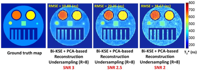
Critical SNR. 8-fold undersampled data was used for reconstruction (127×127 matrix). SNR was iteratively tuned by adjusting noise level to achieve the targeted SNR before performing undersampling. For these experimental conditions, an SNR of 3 is the minimum for acceptable quality reconstruction.
Simulation - Resolution and Acceleration
The fully sampled k-spaces were retrospectively undersampled with different acceleration factors (R) by using the hierarchical random sampling explained in the above section. The data were generated with low SNRs to highlight the performance of the proposed method (5 for 127×127×127, 7 for 95×95×95, and 9 for 61×61×61 k-spaces, when measured at 1100 ns). Data were acquired at R=1, 4, 6, 8 for 61×61×61 k-space; R=8, 12, 15 for 95×95×95; R=15, 30, 60 for 127×127×127 k-space.
Phantom experiment
Details regarding the specifications of the EPRI spectrometer have been previously published (5,28). For the tube phantom experiment, 3D EPR data was obtained using three-tube phantom comprised of three tubes containing 2 mM Oxo-63 (GE Healthcare, Waukesha, WI) bubbled with 0%, 2% and 5% oxygen, respectively. Data was encoded using three orthogonal phase-encoding gradients incrementally ramping in 61 equal steps from −40 to 40 mT m-1, resulting in 61×61×61 phase-encoding steps. 581 data points were encoded with a sampling period of 5ns after the minimum RF recovery dead time (530 ns). 8000 averages per phase encoding point and an interpulse delay (TR) of 10 μs was used. A total of 28,373 points (approximately 8-fold undersampling) with a 61×61×61 matrix size were phase-encoded using the hierarchical random sampling strategy.
Data Processing
Bi-KSE was performed in the peripheral region (Zone 3), and unilateral/backwards KSE was independently performed in the central region (Zone 1 and Zone 2) in a reversely cascading manner, as depicted in Figure 5-a. The extrapolated k-spaces from each phase encoding time delay were individually gridded into Cartesian k-space to generate equal FOV images (Figure 5-b). Then, these images were used as input to the PCA-based reconstruction (Figure 5-c). With a sequence of final images reconstructed by using above-explained methods, T2* was fit using a traditional T2* relaxation model for the magnitude of pixelwise transverse magnetization (Figure 5-d). Linear least-square curve fitting was applied to the log-linearized FID curve in which the slope and the y-intercept represent respectively -1/T2* and log(M0).
Figure 5.

Data processing flowchart. (a) Bilateral k-space (bi-KSE) extrapolation, (b) gridding, (c) PCA-based reconstruction, and (d) pixelwise T2* fitting.
Results
Simulation Results – Undersampling vs. Reduced Averaging
The reconstructed images and the resultant T2* maps obtained using reduced average or undersampling are shown in Figure 6. Reconstructions with gridding are shown in 6a, 6b, 6c for reduced average data, and 6f for undersampled data. KSE is applied to the reduced average data in 6d and 6e, and bi-KSE is applied to the undersampled data in 6g and 6h. PCA-based reconstruction is applied to the reduced average data in 6c and 6e, and to the undersampled data in 6h. As seen in the reconstructed images and the resulting estimated T2* maps, undersampling (6h) outperforms reduced averaging (6c and 6e).
Simulation Results – Resolution and Acceleration
To evaluate how accurately the proposed method estimates T2* with undersampled k-space data, we performed computer simulations using synthesized 3D data consisting of various T2*s (Figure 7-a). In addition to the proposed method, a conventional k-space extrapolation method with full sampling (R=1) was also implemented for comparison. 81 consecutive k-spaces from 700 ns to 1100 ns with a 5 ns time interval were used for reconstruction. Figure 7-b shows the estimated T2* maps obtained using undersampled k-spaces with 61×61×61 gradient steps with acceleration factors of R=1, 4, 6, and 8. Table 1 shows the corresponding quantitative result. Our method enabled accurate T2* estimation up to 8-fold acceleration at this matrix size. However, the small segment E tends to be blurred due to the large voxel size. Figure 8 depicts how the proposed method works with larger matrix sizes. As seen, when higher matrix size is used, the overall performance of our method tends to be improved at the same acceleration factor (R=8) due to the larger central region and higher expected transform sparsity. Moreover, good quality T2* estimation with even higher acceleration factors (R=15 for a 95×95×95 k-space, and R=30 for a 127×127×127 k-space) is attainable.
Table 1.
Quantitative result of estimated T2* for various acceleration factors with 61×61×61 matrix size.
| Segment | A | B | C | D | E | F | |
|---|---|---|---|---|---|---|---|
| R = 8 | mean (ns) | 646.92 | 549.89 | 441.69 | 492.76 | 369.05 | 302.77 |
| standard deviation (ns) | 2.45 | 2.19 | 5.4612 | 0.98 | 2.58 | 8.04 | |
| RMSE (ns) | 3.93 | 2.19 | 9.94 | 7.30 | 31.06 | 8.50 | |
| R = 6 | mean (ns) | 647.27 | 549.59 | 442.97 | 493.15 | 366.94 | 302.04 |
| standard deviation (ns) | 2.35 | 1.94 | 5.65 | 3.36 | 2.69 | 7.91 | |
| RMSE (ns) | 3.60 | 1.98 | 9.01 | 7.62 | 33.16 | 8.17 | |
| R = 4 | mean (ns) | 645.72 | 549.23 | 443.95 | 491.89 | 365.97 | 301.77 |
| standard deviation (ns) | 2.10 | 1.33 | 3.69 | 1.40 | 1.35 | 6.91 | |
| RMSE (ns) | 4.76 | 1.54 | 7.08 | 8.23 | 34.06 | 7.13 | |
| R = 1 | mean (ns) | 649.19 | 550.04 | 448.82 | 500.07 | 383.37 | 302.13 |
| standard deviation (ns) | 5.54 | 3.53 | 4.83 | 3.36 | 2.45 | 6.41 | |
| RMSE (ns) | 5.60 | 3.53 | 4.97 | 3.35 | 16.81 | 6.75 |
The result was evaluated with mean, standard deviation, and root mean square error (RMSE) within each segment. Note that the result shows error of 1% to 2% for the segment A, B, C, D, and F, whereas it shows relatively higher error (around 10%) in segment E. Refer to Figure 7-a for the labeling and corresponding regions.
Figure 8.

Quantitative results with higher matrix sizes. Note that higher matrix size enables higher acceleration factors.
Phantom Experiment Results
Figure 9 shows the T2* map estimated from prospectively undersampled k-spaces (R=8). 91 consecutive k-spaces from 1530 ns to 1980 ns with a 5 ns time interval were used for reconstruction. As seen in Figure 9, the proposed method enables reliable parameter estimation with reduced sampling. The estimate was 684.45 ± 39.10 ns, 659.79 ± 31.11 ns, and 591.10 ± 25.52 ns for tube bubbled with 0%, 2%, and 5% oxygen, respectively, which lie within the our expected range. The estimated numbers show 4%-6% standard deviation, which is presumably due to the system noise in the current EPR scanner. Fitted %oxygen-R2* curve showed slope of 4.68×10⁻⁵ (ns-1 %oxygen-1) and y-intercept of 1.45×10⁻³ (ns-1) with R2=0.9662.
Figure 9.

Estimated T2* map in imaging experiment of three tubes of 2 mM Oxo-63 bubbled with 0%, 2%, and 5% oxygen. Prospectively undersampled (R=8) k-spaces from 1530ns to 1980ns were used for reconstruction. The estimated T2* in each tube is quite homogeneous for the 0% (684.45 ± 39.10 ns), 2% (659.79 ± 31.11 ns), and 5% (591.10 ± 25.52 ns) tubes.
Discussion and Conclusions
The proposed reconstruction method allows significant improvement in the spatial resolution of single point EPRI. For example, if we acquire data with 61×61×61 gradient steps, the full sampling scheme will require a scanning time of approximately 75.7 min (226,981 points × 2,000 averages × 10 μs TR), whereas 8-fold undersampling will enable imaging within approximately 9.5 min (28,373 points). Compared to methods that require multiple gradient acquisitions (typically 3), the proposed technique represents a 24-fold increase in temporal resolution. When using higher matrix size, we were able to achieve higher acceleration factors, for example R=15 with 95×95×95 or R=30 with 127×127×127 gradient steps. Nonetheless, these larger matrix sizes may not be realistic for SP-EPRI since a large number of sampled points are still required, for example 57,158 points and 68,279 points to achieve R=15 with 95×95×95 and R=30 with 127×127×127 matrix size, respectively, which are equivalent to 19.1 min and 22.8 min of scanning time. Such scans might also operate at unrealistic signal to noise levels, despite our methods strong performance with low SNR data (SNRs of 5 for 127×127×127, 7 for 95×95×95, and 9 for 61×61×61 k-spaces, when measured at 1100 ns were utilized). Therefore, choosing a lower resolution (61×61×61) and moderate acceleration (R=8) enables reasonable scanning time (<10 min) but also achieves high spatial resolution to localize hypoxic tissues. However, with the addition of other complimentary fast imaging techniques, such as parallel imaging, further improvements may allow higher resolution image will be able to be obtained within reasonable scanning time, well within the probe clearance time. Improvements in SNR will be aided by the development of phased-array coils (29).
It is not unexpected that undersampling performs better than reduced averaging in SP-EPRI. In our proposed method, the large central region is secured with a hierarchical random sampling pattern, where the sampled k-space is acquired with a higher SNR than full sampling would allow. Even though PCA-constrained reconstruction is applied to both sampling methods, when the SNR falls below a critical threshold noise (and aliasing) is unable to be separated. By applying undersampled acquisitions we can trade recoverable aliasing for improved SNR (16). Note that our simulations comparing reduced averaging to undersampled acquisitions were performed with R=8. For higher acceleration factors, it is not controversial to expect even greater improvements for undersampled acquisitions compared to reduced averaging. Finally, because the KSE techniques propagate k-space points from the periphery of k-space, they perform poorly in instances of low SNR (Figure 6-d and 6-e). This is also not unexpected due to low signal levels in the periphery of k-space with a higher noise floor in the case of reduced averaging.
In this study, we have explored the methods to accelerate EPR imaging without loss of accuracy in the T2*/oxygen quantification. To secure k-space samples as many as possible we have developed the bi-KSE method. Moreover, the model-based reconstruction using PCA has been adapted to further improve the accuracy of T2* estimation. With a computer simulation and phantom experiment, we have verified that the proposed methods enable significant acceleration (8-fold, 15-fold, and 30-fold accelerations respectively for 61×61×61, 95×95×95, and 127×127×127 gradient steps), which realizes more reasonable scan time and higher spatial resolution in the current SP-EPRI system.
Acknowledgments
The authors acknowledge Dr. Rao Gullapalli from the University of Maryland, Baltimore for assistance in performing experiments. Research reported in this publication was supported by the National Institute of Biomedical Imaging and Bioengineering of the National Institutes of Health under Award Number 1R21EB013770. The content is solely the responsibility of the authors and does not necessarily represent the official views of the National Institutes of Health.
References
- 1.Hoek TLV, Becker LB, Shao Z-H, Li C-Q, Schumacker PT. Preconditioning in Cardiomyocytes Protects by Attenuating Oxidant Stress at Reperfusion. Circulation Research. 2000 Mar;86(5):541–548. doi: 10.1161/01.res.86.5.541. [DOI] [PubMed] [Google Scholar]
- 2.Vaupel P, Schlenger K, Knoop C, Hã M. Oxygenation of human tumors: evaluation of tissue oxygen distribution in breast cancers by computerized O2 tension measurements. Cancer research. 1991;51(12):3316–3322. [PubMed] [Google Scholar]
- 3.Rosenman J. Incorporating functiona imaging, information into radiation treatment. Seminars in radiation oncology. 2001;11(1):83–92. doi: 10.1053/srao.2001.18155. [DOI] [PubMed] [Google Scholar]
- 4.Subramanian S, Devasahayam N, Murugesan R, Yamada K, Cook J, Taube A, Mitchell JB, Lohman JaB, Krishna MC. Single-point (constant-time) imaging in radiofrequency Fourier transform electron paramagnetic resonance. Magnetic Resonance in Medicine. 2002 Aug;48(2):370–9. doi: 10.1002/mrm.10199. [DOI] [PubMed] [Google Scholar]
- 5.Devasahayam N, Subramanian S, Murugesan R, Hyodo F, Matsumoto K-I, Mitchell JB, Krishna MC. Strategies for improved temporal and spectral resolution in in vivo oximetric imaging using time-domain EPR. Magnetic Resonance in Medicine. 2007 Apr;57(4):776–83. doi: 10.1002/mrm.21194. [DOI] [PubMed] [Google Scholar]
- 6.Jang H, Subramanian S, Devasahayam N, Saito K, Matsumoto S, Krishna MC, McMillan AB. Single acquisition quantitative single-point electron paramagnetic resonance imaging. Magnetic Resonance in Medicine. 2013 Aug 1;70(4):1173–1181. doi: 10.1002/mrm.24886. [DOI] [PMC free article] [PubMed] [Google Scholar]
- 7.Matsumoto K, Subramanian S, Devasahayam N, Aravalluvan T, Murugesan R, Cook JA, Mitchell JB, Krishna MC. Electron paramagnetic resonance imaging of tumor hypoxia: enhanced spatial and temporal resolution for in vivo pO2 determination. Magnetic Resonance in Medicine. 2006 May;55(5):1157–63. doi: 10.1002/mrm.20872. [DOI] [PubMed] [Google Scholar]
- 8.Hutchinson M, Raff U. Fast MRI data acquisition using multiple detectors. Magnetic Resonance in Medicine. 1988 Jan;6(1):87–91. doi: 10.1002/mrm.1910060110. [DOI] [PubMed] [Google Scholar]
- 9.Sodickson DK, Manning WJ. Simultaneous acquisition of spatial harmonics (SMASH): fast imaging with radiofrequency coil arrays. Magnetic Resonance in Medicine. 1997 Oct;38(4):591–603. doi: 10.1002/mrm.1910380414. [DOI] [PubMed] [Google Scholar]
- 10.Pruessmann KP, Weiger M, Scheidegger MB, Boesiger P. SENSE: sensitivity encoding for fast MRI. Magnetic Resonance in Medicine. 1999 Nov;42(5):952–62. [PubMed] [Google Scholar]
- 11.McGibney G, Smith MR, Nichols ST, Crawley a. Quantitative evaluation of several partial Fourier reconstruction algorithms used in MRI. Magnetic Resonance in Medicine. 1993 Jul;30(1):51–9. doi: 10.1002/mrm.1910300109. [DOI] [PubMed] [Google Scholar]
- 12.Subramanian S, Chandramouli GVR, McMillan A, Gullapalli RP, Devasahayam N, Mitchell JB, Matsumoto S, Krishna MC. Evaluation of partial k-space strategies to speed up time-domain EPR imaging. Magnetic Resonance in Medicine. 2012 Oct 8;70:745–753. doi: 10.1002/mrm.24508. [DOI] [PMC free article] [PubMed] [Google Scholar]
- 13.Lustig M, Donoho D. Compressed sensing MRI. Signal Processing Magazine. 2008 Mar;:72–82. [Google Scholar]
- 14.Donoho DL. Compressed sensing. IEEE Transactions on Information Theory. 2006;52(4):1289–1306. [Google Scholar]
- 15.Candes EJ, Tao T. Near-Optimal Signal Recovery From Random Projections: Universal Encoding Strategies? IEEE Transactions on Information Theory. 2006 Dec;52(12):5406–5425. [Google Scholar]
- 16.Lustig M, Donoho D, Pauly JM. Sparse MRI: The application of compressed sensing for rapid MR imaging. Magnetic Resonance in Medicine. 2007 Dec;58(6):1182–95. doi: 10.1002/mrm.21391. [DOI] [PubMed] [Google Scholar]
- 17.Gamper U, Boesiger P, Kozerke S. Compressed sensing in dynamic MRI. Magnetic Resonance in Medicine. 2008 Feb;59(2):365–73. doi: 10.1002/mrm.21477. [DOI] [PubMed] [Google Scholar]
- 18.Jung H, Sung K, Nayak KS, Kim EY, Ye JC. k-t FOCUSS: a general compressed sensing framework for high resolution dynamic MRI. Magnetic Resonance in Medicine. 2009 Jan;61(1):103–16. doi: 10.1002/mrm.21757. [DOI] [PubMed] [Google Scholar]
- 19.Huang C, Graff CG, Clarkson EW, Bilgin A, Altbach MI. T2 mapping from highly undersampled data by reconstruction of principal component coefficient maps using compressed sensing. Magnetic Resonance in Medicine. 2012 May 16;67(5):1355–66. doi: 10.1002/mrm.23128. [DOI] [PMC free article] [PubMed] [Google Scholar]
- 20.Velikina JV, Alexander AL, Samsonov A. Accelerating MR parameter mapping using sparsity-promoting regularization in parametric dimension. Magnetic Resonance in Medicine. 2013 Nov;70(5):1263–73. doi: 10.1002/mrm.24577. [DOI] [PMC free article] [PubMed] [Google Scholar]
- 21.Aharon M, Elad M, Bruckstein A. K -SVD : An Algorithm for Designing Overcomplete Dictionaries for Sparse Representation. IEEE Transactions on Signal Processing. 2006;54(11):4311–4322. [Google Scholar]
- 22.Doneva M, Börnert P, Eggers H, Stehning C, Sénégas J, Mertins A. Compressed sensing reconstruction for magnetic resonance parameter mapping. Magnetic Resonance in Medicine. 2010 Oct;64(4):1114–20. doi: 10.1002/mrm.22483. [DOI] [PubMed] [Google Scholar]
- 23.Gonzalez R, Woods R. Digital Image Processing. 2. Upper Saddle River, New Jersey: Prentice-Hall, Inc.; 2002. Sharpening Spatial Filters; pp. 75–146. [Google Scholar]
- 24.Beatty PJ, Nishimura DG, Pauly JM. Rapid gridding reconstruction with a minimal oversampling ratio. IEEE transactions on medical imaging. 2005 Jun;24(6):799–808. doi: 10.1109/TMI.2005.848376. [DOI] [PubMed] [Google Scholar]
- 25.Pipe JG. Reconstructing MR images from undersampled data: data-weighting considerations. Magnetic Resonance in Medicine. 2000 Jun;43(6):867–75. doi: 10.1002/1522-2594(200006)43:6<867::aid-mrm13>3.0.co;2-2. [DOI] [PubMed] [Google Scholar]
- 26.Pipe JG, Menon P. Sampling density compensation in MRI: rationale and an iterative numerical solution. Magnetic Resonance in Medicine. 1999 Jan;41(1):179–86. doi: 10.1002/(sici)1522-2594(199901)41:1<179::aid-mrm25>3.0.co;2-v. [DOI] [PubMed] [Google Scholar]
- 27.Rudin L, Osher S, Fatemi E. Nonlinear total variation based noise removal algorithms. Physica D: Nonlinear Phenomena. 1992;60:259–268. [Google Scholar]
- 28.Subramanian S, Devasahayam N, McMillan A, Matsumoto S, Munasinghe JP, Saito K, Mitchell JB, Chandramouli GVR, Krishna MC. Reporting of quantitative oxygen mapping in EPR imaging. Journal of Magnetic Resonance. 2012 Jan;214(1):244–51. doi: 10.1016/j.jmr.2011.11.013. [DOI] [PMC free article] [PubMed] [Google Scholar]
- 29.Enomoto A, Hirata H, Matsumoto S, Saito K, Subramanian S, Krishna MC, Devasahayam N. Four-channel surface coil array for 300-MHz pulsed EPR imaging: Proof-of-concept experiments. Magnetic Resonance in Medicine. 2014 Mar 26;71(2):853–858. doi: 10.1002/mrm.24702. [DOI] [PMC free article] [PubMed] [Google Scholar]