Differential diagnosis of neurodegenerative diseases using structural MRI data

Juha Koikkalainen; Hanneke Rhodius-Meester; Antti Tolonen; Frederik Barkhof; Betty Tijms; Afina W Lemstra; Tong Tong; Ricardo Guerrero; Andreas Schuh; Christian Ledig; Daniel Rueckert; Hilkka Soininen; Anne M Remes; Gunhild Waldemar; Steen Hasselbalch; Patrizia Mecocci; Wiesje van der Flier; Jyrki Lötjönen

doi:10.1016/j.nicl.2016.02.019

. 2016 Mar 5;11:435–449. doi: 10.1016/j.nicl.2016.02.019

Differential diagnosis of neurodegenerative diseases using structural MRI data

Juha Koikkalainen ^a,^i,^⁎, Hanneke Rhodius-Meester ^b, Antti Tolonen ^a, Frederik Barkhof ^c, Betty Tijms ^b, Afina W Lemstra ^b, Tong Tong ^d, Ricardo Guerrero ^d, Andreas Schuh ^d, Christian Ledig ^d, Daniel Rueckert ^d, Hilkka Soininen ^e, Anne M Remes ^e, Gunhild Waldemar ^g, Steen Hasselbalch ^g, Patrizia Mecocci ^h, Wiesje van der Flier ^b,^f, Jyrki Lötjönen ^a,ⁱ

PMCID: PMC4827727 PMID: 27104138

Abstract

Different neurodegenerative diseases can cause memory disorders and other cognitive impairments. The early detection and the stratification of patients according to the underlying disease are essential for an efficient approach to this healthcare challenge. This emphasizes the importance of differential diagnostics. Most studies compare patients and controls, or Alzheimer's disease with one other type of dementia. Such a bilateral comparison does not resemble clinical practice, where a clinician is faced with a number of different possible types of dementia.

Here we studied which features in structural magnetic resonance imaging (MRI) scans could best distinguish four types of dementia, Alzheimer's disease, frontotemporal dementia, vascular dementia, and dementia with Lewy bodies, and control subjects. We extracted an extensive set of features quantifying volumetric and morphometric characteristics from T1 images, and vascular characteristics from FLAIR images. Classification was performed using a multi-class classifier based on Disease State Index methodology. The classifier provided continuous probability indices for each disease to support clinical decision making.

A dataset of 504 individuals was used for evaluation. The cross-validated classification accuracy was 70.6% and balanced accuracy was 69.1% for the five disease groups using only automatically determined MRI features. Vascular dementia patients could be detected with high sensitivity (96%) using features from FLAIR images. Controls (sensitivity 82%) and Alzheimer's disease patients (sensitivity 74%) could be accurately classified using T1-based features, whereas the most difficult group was the dementia with Lewy bodies (sensitivity 32%). These results were notable better than the classification accuracies obtained with visual MRI ratings (accuracy 44.6%, balanced accuracy 51.6%). Different quantification methods provided complementary information, and consequently, the best results were obtained by utilizing several quantification methods.

The results prove that automatic quantification methods and computerized decision support methods are feasible for clinical practice and provide comprehensive information that may help clinicians in the diagnosis making.

Keywords: MRI, Neurodegenerative diseases, Classification, Volumetry, TBM, VBM, Alzheimer's disease, Frontotemporal lobar degeneration, Vascular dementia, Dementia with Lewy bodies

Graphical abstract

Highlights

•
Differential diagnostics of dementias was studied using structural MRI data.
•
504 patients with both T1 and FLAIR MRIs from five patient classes were evaluated.
•
Different fully automatic quantification methods were compared and combined.
•
Classification accuracy of 70.6% was obtained for 5-class classification problem.
•
Combination of several quantification methods was needed for optimal accuracy.

1. Introduction

Dementia is a general term to describe a syndrome involving loss of cognitive abilities. Most often dementia is caused by a progressive neurodegenerative disease. Dementia is a major health issue in our society both from the economic and human point of view.

Alzheimer's disease (AD) is the most common type of dementia that may account for 60–75% of dementia cases. Vascular dementia (VaD) and dementia with Lewy bodies (DLB) also occur frequently in elderly patients, while frontotemporal dementia (FTD) is relatively more common in dementia patients with early onset. Characteristic structural pathologies in these diseases include atrophy of the medial temporal lobe in AD and atrophy of the frontal and temporal lobes in FTD. In DLB the brain structure is typically less affected. Absence of medial temporal lobe atrophy and findings of infarcts or white matter changes are typical to VaD. The atrophy patterns can be detected with T1-weighted images. Cortical and lacunar infarcts and white matter changes that are typical to VaD are identified on T1-weighted images and T2-weighted, dual-echo Turbo Spin Echo (TSE) or Fluid-Attenuated Inversion Recovery (FLAIR) images.

Early and accurate differential diagnostics of neurodegenerative diseases is essential for two reasons. First, it has been shown that early diagnosis combined with current treatments can delay hospitalization (Feldman et al., 2009), and the importance of the early diagnosis will dramatically increase as soon as disease-modifying drugs become available (Siemers et al., 2015). Second, developing new treatments requires early and accurate identification of correct target populations. It has been hypothesized that too heterogeneous study populations may explain the failure of some previous pharmaceutical trials (Falahati et al., 2014).

The studies on structural MRI that have characterized distinct neurodegenerative diseases are mostly based on visual ratings (Barber et al., 1999, Burton et al., 2009, Meyer et al., 2007, Varma et al., 2002), volumetry (Meyer et al., 2007, Frisoni et al., 1999, Barber et al., 2000, Munoz-Ruiz et al., 2012, Ishii et al., 2007), and local morphometry analyses (Munoz-Ruiz et al., 2012, Laakso et al., 2000, Burton et al., 2002, Barber et al., 2002, Ballmaier et al., 2004, Whitwell et al., 2007, Rabinovici et al., 2008, Klöppel et al., 2008). Typical findings on the differences between different dementia types include: 1) the hippocampal volume and medial temporal lobe are relatively preserved in FTD as compared to AD (Duara et al., 1999, Frisoni et al., 1999), 2) FTD-specific atrophy of the frontal and temporal lobes (Duara et al., 1999, Varma et al., 2002, Klöppel et al., 2008), 3) relatively preserved brain anatomy in DLB as compared to AD and FTD (Meyer et al., 2007, Barber et al., 1999, Barber et al., 2000, Burton et al., 2002, Burton et al., 2009, Kantarci et al., 2012, Ishii et al., 2007, Whitwell et al., 2007), and 4) extensive white matter changes with lacunar and cortical infarcts in VaD (Meyer et al., 2007).

There are extensive literature comparing the dementia types with controls, but far less studies have been done on comparing the different dementia types with each other. In clinical practice, the actual question is to determine to which type of dementia a patient with cognitive complaints should be diagnosed. The guidelines for the early detection of neurodegenerative diseases (Román et al., 1993, Neary et al., 1998, McKeith et al., 2005, Dubois et al., 2007, Waldemar et al., 2007, McKhann et al., 2011) are relatively general and do not provide specific and uniform information for accurate differential diagnostics of neurodegenerative diseases. Therefore, the current diagnostic processes involve a certain degree of subjective assessment and require significant expertise from clinicians. Automatic image quantification methods and computerized decision support methods are able to objectively extract lots of information, more than the human eye can see, and evaluate how the patient data relates to typical data from different dementias. Such data are likely to be useful in clinical diagnosis making, especially supporting the decisions of unexperienced clinicians.

The objective of this paper is to perform an extensive study on differential diagnostics of dementias utilizing only structural MRI data. We evaluate several state of the art automatic quantification methods in order to find out which of the methods or what combination gives optimal classification accuracy. We utilize a dataset of 504 patients divided into five different groups: controls (CN), AD, FTD, DLB, and VaD. Both T1 and FLAIR data are used in the analysis.

2. Material and methods

2.1. Patient groups

We study a total of 504 patients from the Amsterdam Dementia Cohort who had visited the Alzheimer center of the VU University Medical Center between 2004 and 2014 (van der Flier et al., 2014). The patients were included if MRI and mini mental state examination (MMSE) (Folstein et al., 1975) were present. At baseline, all patients received a standardized and multi-disciplinary work-up, including medical history, physical, neurological and neuropsychological examination, MRI, laboratory test and lumbar puncture to collect cerebrospinal fluid. Diagnoses were made in a multidisciplinary consensus meeting.

In this study, patients with subjective cognitive decline (SCD) were regarded as the control subjects. Patients were diagnosed as having SCD when cognitive complaints could not be confirmed by cognitive testing and criteria for MCI, dementia or other neurological or psychiatric disorder known to cause cognitive complaints were not met. Patients were diagnosed with probable AD using the criteria of the National Institute for Neurological and Communicative Diseases Alzheimer's Disease and Related Disorders Association; all patients also met the core clinical criteria of the National Institute on Aging-Alzheimer's Association guidelines for AD (McKhann et al., 1984, McKhann et al., 2011). FTD was diagnosed using the Neary criteria; patients also met the core criteria from Rasckovsky (Neary et al., 1998, Rascovsky et al., 2011). VaD was diagnosed using the National Institute of Neurological Disorders and Stroke and Association Internationale pour la Recherché et l'Enseignement en Neurosciences criteria (Román et al., 1993), and DLB using the McKeith criteria (McKeith et al., 1996, McKeith et al., 2005). The study was approved by the local Medical Ethical Committee. All patients have signed written informed consent for their clinical data to be used for research purposes.

The normal cognition of all the SCD patients was confirmed at 9 months follow-up. Follow-up took place by annual routine visits to the memory clinic in which patient history, cognitive tests and a general physical and neurologic examination were repeated. Follow-up data was available in all SCD subjects, with a mean of 2.5 ± 1.4 years.

2.2. Imaging

Subjects were scanned routinely on either 1.0 T, 1.5 T or 3.0 T MRI devices. All scans include a 3-dimensional T1-weighted gradient echo sequence and a fast FLAIR sequence. The voxel size of the T1-images varies between 0.9 × 0.9 × 0.9 mm³ and 1.1 × 1.1 × 1.5 mm³. For FLAIR images there is much more variation in the slice thickness, as the voxel size varies between 0.4 × 0.4 × 1.0 mm³ and 1.2 × 1.2 × 5.0 mm³. 86 patients were imaged using 1.0 T device, whereas 1.5 T and 3.0 T devices were used for the remaining 97 and 321 patients, respectively. Detailed information on the imaging parameters for each disease group is available in Appendix A.

Imaging data were assessed visually for atrophy and vascular changes. Visual rating of medial temporal lobe atrophy was performed on coronal T1-weighted images according to the 5-point (0–4) rating scale for medial temporal lobe atrophy (MTA) from the average score of the left and right sides (Scheltens et al., 1995). Global cortical atrophy (GCA) was assessed visually on axial FLAIR images (possible range of scores 0–3) (Pasquier et al., 1996). The degree of severity of white matter hyperintensities was rated on axial FLAIR images using Fazekas' scale (possible range of scores 0–3) (Fazekas et al., 1987). The number of lacunes (# of lacunes) was defined as T1-hypointense and T2-hyperintense CSF-like lesions surrounded by white matter or subcortical gray matter. Next to an overall count of lacunes, the presence of ≥ 1 lacunes in the basal ganglia (BG lacunes) was determined. Finally, the presence of infarcts ≥ 1 (Infarcts) was visually evaluated.

In this study, the visual scores serve as reference values: the multi-class classification is performed using visual scores (Section 3.1) and the results obtained with automatic image quantification methods (Section 3.2) are compared against these results.

2.3. Atlases and templates

Automated image quantification tools used in this work require atlas data. For this purpose we use a set of 60 subjects from the ADNI database (http://adni.loni.usc.edu/), consisting of 20 elderly healthy controls, 20 mild-cognitive impairment subjects and 20 AD subjects. For each atlas image (T1 MR images of the 60 subjects), a whole brain segmentation (http://www.neuromorphometrics.com/) containing 139 regions (98 cortical parcellations and 41 sub-cortical regions) was generated. In addition, in order to produce more accurate segmentations for hippocampus, the semi-automatic hippocampus segmentations of the ADNI database are used as atlas segmentations as done in (Lötjönen et al., 2010, Lötjönen et al., 2011).

A mean anatomical template generated from 30 ADNI images is used as the reference image in the morphometric analyses (Guimond et al., 2000, Koikkalainen et al., 2011).

2.4. Image quantification methods

Several fully automatic image quantification methods are tested to quantify different aspects of images: 1) volumetry using multi-atlas segmentation, 2) atrophy of brain tissue using voxel-based morphometry (VBM) and tensor-based morphometry (TBM), 3) similarities with database images using manifold learning and ROI-based grading, and 4) vascular changes by segmentation of white matter hyperintensities and cortical and lacunar infarcts.

2.4.1. Pre-processing

T1-weighted images are first re-sampled to 1 mm isotropic voxels. Then, the images are skull-stripped, bias field corrected, and intensities normalized using in-house software tools. The segmentation of brain tissue into white matter (WM), grey matter (GM), and cerebrospinal fluid (CSF) is done based on the Expectation-Maximization (EM) algorithm (Leemput et al., 1999).

FLAIR images are bias corrected using ITK's N4 bias field correction algorithm (Tustison et al., 2010). For the registration of T1 and FLAIR images, the FLAIR images are re-sampled to 1 mm isotropic voxels. After that, T1 images are registered to FLAIR images by maximizing Normalized Mutual Information (NMI) (Studholme et al., 1999) using gradient ascent. This transformation is used to transform the results of the T1 images to FLAIR coordinates.

2.4.2. Multi-atlas segmentation

Multi-atlas segmentation methods have been proven to produce robust and accurate segmentations of brain structures (Heckemann et al., 2006, Aljabar et al., 2009, Lötjönen et al., 2010, van Rikxoort et al., 2010). In this study, multi-atlas segmentation is used to segment hippocampus and to segment the whole brain into 139 regions using the atlases presented in Section 2.3.

The segmentation method is presented in (Lötjönen et al., 2010, Lötjönen et al., 2011) and was extended by local weighting of atlases (Artaechevarria et al., 2009). In this method, the T1 image of a patient and the atlases are first registered using coarse non-rigid deformation. Then, an atlas selection is used to select 12 atlases out of the 60 atlases for more detailed non-rigid registration. A probabilistic atlas, generated from these atlas segmentations, is used as a prior in the intensity-based classification using the EM algorithm (Lötjönen et al., 2010). An example of the segmentation results is given in Fig. 1.

Fig. 1 — An example of the segmentations of T1 MR image.

The following volumetric features are obtained from the multi-atlas segmentation: volumes of left and right hippocampus and the total hippocampal volume, and the volumes of 139 brain regions.

2.4.3. Voxel-based morphometry

VBM is a technique where the local concentration of GM is measured after accounting for global differences in anatomy by registering a patient image to a reference image (Ashburner and Friston, 2000).

In VBM, the registration of the patient's T1 image to the reference image is usually performed using a coarse non-linear registration approach. Here, registration parameters that result in a coarse match of the reference and patient images are used. Further details regarding the registration method used can be found in (Lötjönen et al., 2010). The GM segmentation of the patient is propagated to the reference space according to the calculated transformation. The GM segmentation is then smoothed using a Gaussian filter (σ = 4 mm) to produce a measure of GM concentration for each voxel.

In order to generate a relatively small set of easily interpretable features for classification, the features are computed by combining the data within each of 139 regions of interest (ROIs). In addition, a global feature for the whole brain is computed by using the whole brain as a ROI. If the GM concentration is simply averaged ROI-wise, there can be inside a ROI both voxels where the GM concentration is higher in one disease group as compared to the other, and voxels where the GM concentration is lower. Consequently, the averaging would cancel these two opposite effects. Because of this, the GM concentration is computed separately for the voxels with typically higher or lower GM concentration, and then these values are summed up with different signs:

F_{i, j}^{VBM} (R) = \frac{\sum_{\vec{p} \in R \cap (T_{i, j} (\vec{p}) > 0)} W (\vec{p}) \cdot GM (\vec{p}) - \sum_{\vec{p} \in R \cap (T_{i, j} (\vec{p}) < 0)} W (\vec{p}) \cdot GM (\vec{p})}{\sum_{\vec{p} \in R} W (\vec{p})},

(1)

where R defines the ROI, i and j define the two diseases studied, $GM (\vec{p})$ is the GM concentration for voxel $\vec{p}$ , $T_{i, j} (\vec{p})$ is the t-value from the group-level t-test (comparison of the two diseases), and $W (\vec{p})$ is a weighting function defined as

W (\vec{p}) = \{\begin{cases} 1, & if P_{i, j} (\vec{p}) < 0.000001 \\ 0, & if P_{i, j} (\vec{p}) > 0.05 \\ \frac{log (0.05) - log (P_{i, j} (\vec{p}))}{log (0.05) - log (0.000001)}, & otherwise \end{cases}),

(2)

where $P_{i, j} (\vec{p})$ is the p-value of the t-test. Note that the VBM features are computed for each pair-wise comparison of two diseases in order to extract information only from those regions with relevant information for the particular pair of diseases. The p- and t-values are computed by applying the t-test on GM concentration data of a separate training set consisting of patients from the two disease groups i and j.

Consequently, 139 ROI-wise and one global VBM features are obtained for each pair-wise comparison of diseases, i.e., in total 20 sets of VBM features for five groups. Note that F_i , j^VBM(R) = - F_j , i^VBM(R), so in practice only 10 sets of features need to be computed.

2.4.4. Tensor-based morphometry

An alternative approach to VBM is to characterize differences in brain morphometry using TBM. In TBM, the reference image is registered to the patient image using high-dimensional registration, and the analysis is done by comparing measures derived from the deformation fields (Ashburner et al., 1998). In this study, the same registration method that is used in VBM is used in the TBM analysis, but the parameters are chosen to perform the registration at a finer level of detail. The local volume difference as compared to the reference is used to quantify the non-rigid deformation by computing the determinant of the Jacobian matrix:

J (\vec{p}) = |\begin{array}{c} \frac{\partial D_{x} (\vec{p})}{\partial x} & \frac{\partial D_{x} (\vec{p})}{\partial y} & \frac{\partial D_{x} (\vec{p})}{\partial z} \\ \frac{\partial D_{y} (\vec{p})}{\partial x} & \frac{\partial D_{y} (\vec{p})}{\partial y} & \frac{\partial D_{y} (\vec{p})}{\partial z} \\ \frac{\partial D_{z} (\vec{p})}{\partial x} & \frac{\partial D_{z} (\vec{p})}{\partial y} & \frac{\partial D_{z} (\vec{p})}{\partial z} \end{array}|,

(3)

where $D_{x} (\vec{p})$ , $D_{y} (\vec{p})$ , and $D_{z} (\vec{p})$ give the deformation from the reference to the patient image in x-, y-, and z-directions for voxel $\vec{p}$ .

The features are computed as in the VBM analysis. The only difference is that the GM concentration in Eq. (1) is replaced by the logarithm of the Jacobian $log (J (\vec{p}))$ . The logarithm is used to make the Jacobians more normally distributed and treat contraction and expansion in a similar fashion. As in the VBM analysis, the t-test is applied to a training set to produce t- and p-values for the feature computation. The TBM analysis produces in total 140 features for each comparison of two diseases.

2.4.5. Manifold learning

A fundamental problem when dealing with high-dimensional data such as 3D brain MR images is the large amount of variables (for example, over 16 million voxels for a 256 × 256 × 256 image) available in images, where not all contain equal (or any) desired information. Manifold learning aims at finding a low-dimensional representation of high-dimensional data while trying to faithfully represent the intrinsic local geometry of the data. In (Guerrero et al., 2014, Wolz et al., 2011) manifold learning was used in the context of neurodegenerative disease population modeling to extract a meaningful low-dimensional representation better suited for classification.

Laplacian eigenmaps (Belkin and Niyogi, 2002) can be used to derive a mapping from a high-dimensional space $R^{D}$ to a low-dimensional space $R^{d}$ that best represents a population X, such that d ≪ D. Here local geometry is determined by converting pairwise sum of squared differences (SSD) to a similarity matrix G using a Gaussian heat kernel. From G, the k-neighborhoods of data points are used to construct a sparse neighborhood matrix W. Laplacian eigenmaps seeks to place points x_s and x_r close together in $R^{d}$ if they are close in the original $R^{D}$ space (large similarity w_s , r). This is achieved by means of minimizing ϕ(Y) = argmin ∑_s , r‍ ∥ y_s - y_r ∥²w_s , r under the constraint that y^TLy = 1, where y are the calculated manifold coordinates. This can be formulated as generalized eigenproblem Lν = μMν, where L = M - W is the graph Laplacian and M is a degree matrix. Here ν and μ are the eigenvectors and eigenvalues, where the d eigenvectors corresponding to the smallest (non-zero) eigenvalues represent the new coordinate system.

In this study two ROIs are utilized in manifold learning: one for hippocampus region and one for frontotemporal lobe region (Fig. 2). The ROIs were generated by dilating ten times the segmentations for hippocampus and temporal pole. In the classification, ten eigenvectors are used, consequently resulting in ten features for both ROIs.

2.4.6. ROI-based grading

In ROI-based grading, the idea is to propagate disease labels of training subjects to test subjects and assign disease scores for the test subjects. Given the training population, the relationship between each test subject and the training population is investigated so that the disease information of the training population can be propagated to test subjects. The grading features are calculated based on the methods proposed in (Coupé et al., 2012, Tong et al., 2013).

In (Coupé et al., 2012), the relationship is modeled using a weighting function. Here, we model this relationship using a sparse representation method, which has been demonstrated to be superior to the weighting function in image segmentation (Tong et al., 2013). Data of each test subject is assumed to lie in the space of the training population and be represented by a linear combination of the data from few training subjects. In order to seek a sparse representation of the data of each test subject, we utilize the Elastic Net sparse coding technique as in (Tong et al., 2013). Given the intensities of a test subject X_test ∈ R^k × 1 and the intensities of n training subjects X_training ∈ R^k × n in a ROI, the grading score g_test of this test subject can be calculated by minimizing the following cost function:

\{\begin{cases} \hat{α} = min_{α} \frac{1}{2} | | X_{test} - X_{training} α | |_{2}^{2} + λ_{1} | | α | |_{1} + \frac{λ_{2}}{2} | | α | |_{2}^{2} \\ g_{test} = \frac{\sum_{s = 1}^{n} {\hat{α}}_{t} (s) l_{s}}{\sum_{s = 1}^{n} {\hat{α}}_{t} (s)} . \end{cases})

(4)

Here $\hat{α}$ are the coding coefficients of the test subject and l_s is the disease label vector for the sth training subject. Each training label vector is defined as l_s = [0, 0 … 1 … 0, 0], where the non-zero entry position indicates the disease label of a specific group. Most of the coefficients in $\hat{α}$ are zero due to the sparsity constraint. If the sth coefficient in $\hat{α}$ is not zero, it indicates that the corresponding sth training subject has been selected to propagate its clinical label information to the test subject. Finally, the calculated grading scores can be used as features for classification. The same ROIs that are used in manifold learning are used also in ROI-based grading.

2.4.7. Segmentation of white matter hyperintensities

The segmentation of white matter hyperintensities (WMH) is done according to the method presented in (Wang et al., 2012). The method is based on the EM algorithm, and the segmentation is done in three steps:

1.
Segment WM in two classes from T1 image representing hypointense WM regions in T1 image and normal bright WM regions.
2.
Using the results of the previous step as an initialization, segment the FLAIR image to three classes: CSF, normal brain tissue, and hyperintense voxels.
3.
Using the results of the previous step as an initialization, segment the WM and subcortical regions from the FLAIR image in two classes. The class with higher intensities was then regarded as the segmentation of WMH.

The segmentations of WM, CSF, and subcortical regions are obtained from the segmentation of T1 image (2.4.1, 2.4.2). An example of the WMH segmentation is shown in Fig. 3.

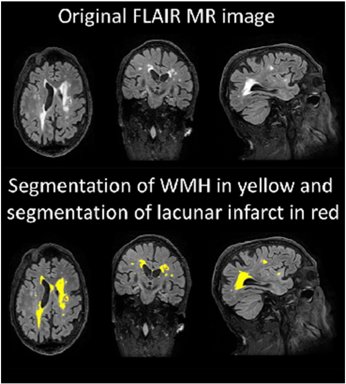
Fig. 3 — An example of segmentation of a FLAIR image.

Instead of the raw total WMH volume, a masked WMH volume is computed in order to provide better discriminatory information. A mask was generated that includes only voxels that are brighter than the 99.3% percentile of the intensities inside the brain and are located inside the centrum semiovale. The masked WMH volume is computed as the WMH volume inside the mask. The parameter for the threshold was determined by testing several values. The centrum semiovale was defined from the MNI 152-template: first, the white matter superior to the lateral ventricles (z > 32) was extracted, and then the sulcal white matter regions were removed using a set of morphological operations. The segmentation of centrum semiovale is propagated to the patient images based on MNI-to-reference and reference-to-patient registrations.

2.4.8. Segmentation of cortical infacortical infarcts

Cortical infarcts are segmented as the hyperintense regions in FLAIR images that are partly located in cortex. The segmentation of the cortex is obtained from the multi-atlas segmentation of the T1 image (Section 2.4.2, segmentation method evaluated in (Lötjönen et al., 2010, Lötjönen et al., 2011)) and the threshold for the segmentation is computed utilizing the WMH segmentation. The total volume of cortical infarcts is computed from the segmentation.

2.4.9. Segmentation of lacunar infarcts

A method was developed for the segmentation of lacunar infarcts utilizing both FLAIR and T1 images. The method first detects candidate locations via localizing “holes” in a T1 image, and then classifies these holes based on the intensities and contrasts in T1 and FLAIR images.

In order to find the holes, the tissue segmentation of T1 image is performed using two approaches: 1) EM-based classification and 2) multi-atlas segmentation as in Section 2.4.2. EM-classification is based mostly on the voxel intensities, i.e., a voxel with low intensity is typically classified as CSF. On the other hand, small holes get easily misclassified in multi-atlas segmentation if they are in the middle of WM and a strong probabilistic prior term is used. Consequently, holes can be detected as the voxels that are classified as CSF in EM-classification and as WM or GM in multi-atlas segmentation.

A hole is classified as a lacunar infarct if 1) in FLAIR, the contrast of the hole and the surrounding tissue is large, 2) the surrounding tissue in FLAIR is bright, and 3) the intensity in T1 image is low. However, in basal ganglia the condition 2 is not expected. Finally, only the infarcts with diameter larger than 3 mm and smaller than 15 mm are regarded as lacunar infarcts.

2.4.10. Vascular burden measure

The clinical criteria for the diagnosis of VaD include evidence of infarcts, lacunar infarcts, and white matter lesions (Román et al., 1993), but all of these findings are not needed for the diagnosis. To mimic these criteria, a vascular burden measure is computed to take into account the fact that, for example, a patient with no lacunar infarcts can be diagnosed as VaD:

Vascular burden = masked WMH volume + volume of cortical infarcts + 300 \cdot volume of lacunar infarcts .

(5)

In other words, all the volumes are summed up, but because of the small volume of the lacunar infarcts they are given an empirically determined larger weight. This measure is used as a classification feature.

2.5. Normalization of features

The classification features are adjusted for covariates to take into account normal age- and gender-related differences. The covariate adjustment is performed by fitting a multi-dimensional linear regression model to the distribution of the feature values of the control group using age and gender as independent variables. Only control data are used here so that any disease-related effects would not be removed. The feature values of each patient are then normalized using the obtained regression parameters according to patient's age and gender (Koikkalainen et al., 2012).

In addition, it was noticed that the images acquired with the 1.0 T MRI device produce systematic differences as compared to the remaining images. Consequently, an additional binary independent variable is added to the normalization that removes this systematic error from the feature values and makes it possible to simultaneously analyze images acquired with different MRI devices.

2.6. Classification

The classification based on the quantified MRI biomarkers is performed using a modification of the Disease State Index (DSI) classifier (Mattila et al., 2011, Mattila et al., 2012) that has been originally developed for two-class problems. For this application, the classifier is modified for multi-class classification. The classifier is described in detail in Appendix B. The classifier gives as an output a continuous index between zero and one, DSI(i, j), for each comparison of two classes i and j. This index describes the likelihood that the patient belongs to class j when class i is an alternative option. From these pair-wise DSI values, total DSI values DSI(i) are computed describing the likelihood that the patient belongs to the class i. Finally, the patient is assigned to the class with the highest index value.

2.7. Evaluation

The classification accuracy is evaluated using 10-fold cross-validation. In practice, 10 percent of the patients are randomly selected as a test set, and the remaining 90% are used as a training set. The training set is used to compute the t-tests needed for the computation of VBM and TBM features (Eqs. (1), (2)), to compute the ROI-based grading features, and to compute the normalization parameters (Section 2.5). In addition, the classifier is trained using the features of the training set and then applied to the test set. This is repeated ten times so that each patient is once used in the test set.

The classification results of the test set are compared to the clinical diagnoses using two measures: classification accuracy (acc) and balanced accuracy (Brodersen et al., 2010) (Bacc):

acc = \frac{\sum_{i = 1}^{N_{c}} # of correctly classified patients of disease i}{# of all patients},

(6)

Bacc = \frac{1}{N_{c}} \sum_{i = 1}^{N_{c}} \frac{# of correctly classified patients of disease i}{# of patients with disease i} .

(7)

The balanced accuracy is used to take into account the imbalance in the number of cases between different classes, reflecting the prevalence of diseases. For example, the training data of this study contains more AD patients than FTD, DLB and VaD patients altogether leading to the situation that classifying all patients as AD produces already relatively good classification accuracy. The balanced accuracy is an estimate of the accuracy the classifier would achieve on a data set consisting of an equal amount of patients in each class.

Because the vascular changes are characteristics to VaD, and there are no VaD specific structural changes, only the vascular burden measure is included in the training set for the VaD patients. In practice this means that the classifier does not use structural features when VaD is one of the two diseases compared. However, all the data are used for the VaD training patients in the evaluations where the vascular burden measure is not used in order to enable fair comparison between methods. For example, when evaluating the performance of VBM alone, the VBM data are used for the VaD training patients. Otherwise, there would be no data for VaD patients in the training set and consequently all VaD patients in the test set would be misclassified.

Also in the ROI-based grading the VaD training data are not used, and consequently the number of features for each ROI is four. For TBM and VBM training data, only the features from the pair-wise comparison F_i , j^VBM/TBM are used when the DSI(i, j) is computed. The training set features used to compute each DSI(i, j) are summarized in Table 1. However, for the test set patients the full set of features is always given to the classifier.

Table 1.

A summary of the training set features used to compute the DSI(i, j) for each disease-pair.

	Features	Description
Volumes	142	Left, right and total hippocampus, 139 regions from atlas
TBM	140	For each disease-pair comparison features for 139 ROIs and a global feature
VBM	140	For each disease-pair comparison features for 139 ROIs and a global feature
Manifold learning	20	Number of manifold dimensions (10) × number of ROIs (2)
ROI-based grading	8	Number of classes (4) × number of ROIs (2)
Vascular burden	1	Vascular burden measure

Open in a new tab

In order to compare the performance of the automatically determined features with the visual MRI ratings, the DSI classifier is also used to classify the patients by utilizing the raw values of the visual MRI ratings as the classification features.

3. Results

3.1. Clinical data and visual MRI ratings

The summary of clinical data and visual MRI ratings is presented in Table 2.

Table 2.

Clinical data and visual MRI ratings for the patient groups. Data presented in mean ± standard deviation or number (percentage). MTA = Medial temporal lobe atrophy, GCA = Global cortical atrophy, # of lacunes = number of lacunar infarcts, BG lacunes = presence of lacunar infarcts in basal ganglia.

	Total	CN	AD	FTD	DLB	VaD
N	504	118	223	92	47	24
Age	64 ± 8	60 ± 8^b^,^c^,^d^,^e	66 ± 7^a^,^c	63 ± 7^a^,^b^,^d^,^e	68 ± 9^a^,^c	68 ± 6^a^,^c
Females	221 (44%)	45 (38%)^b^,^d	120 (54%)^a^,^d	41 (44%)^d	6 (13%)^a^,^b^,^c^,^e	9 (38%)^d
MMSE	23 ± 5	28 ± 1^b^,^c^,^d^,^e	21 ± 5^a^,^c^,^d^,^e	25 ± 5^a^,^b	23 ± 4^a^,^b	24 ± 5^a^,^b
MTA	1.1 ± 0.9	0.3 ± 0.5^b^,^c^,^d^,^e	1.3 ± 0.8^a^,^c^,^d	1.8 ± 1.0^a^,^b^,^d^,^e	0.8 ± 0.7^a^,^b^,^c^,^e	1.3 ± 0.9^a^,^c^,^d
GCA	0.9 ± 0.7	0.3 ± 0.5^b^,^c^,^d^,^e	1.0 ± 0.6^a	1.2 ± 0.8^a	1.0 ± 0.7^a	0.8 ± 0.7^a
Fazekas	0.9 ± 0.9	0.6 ± 0.7^b^,^d^,^e	1.0 ± 0.8^a^,^c^,^e	0.7 ± 0.8^b^,^d^,^e	0.9 ± 0.7^a^,^c^,^e	2.4 ± 0.8^a^,^b^,^c^,^d
# of lacunes	0.3 ± 1.7	0.1 ± 0.3^e	0.2 ± 1.5^e	0.2 ± .0.8^e	0.0 ± 0.2^e	4.3 ± 4.5^a^,^b^,^c^,^d
BG lacunes	31 (6%)	5 (4%)^e	6 (3%)^e	3 (3%)^e	2 (4%)^e	15 (63%)^a^,^b^,^c^,^d
Infarcts	16 (3%)	1 (1%)^e	15 (2%)^e	2 (2%)^e	0 (0%)^e	8 (33%)^a^,^b^,^c^,^d

Open in a new tab

Statistically significant (p < 0.05) differences between the patient groups were studied using the Mann-Whitney U test for age, MMSE, MTA, GCA, Fazekas rating, and number of lacunes.

Chi-squared test was used for the gender, presence of lacunes in basal ganglia and presence of infarcts.

Statistically significantly different from CN.

Statistically significantly different from AD.

Statistically significantly different from FTD.

Statistically significantly different from DLB.

Statistically significantly different from VaD.

The control and FTD groups are the youngest ones, whereas the DLB patients are mostly males. The highest proportion of females is in the AD group. The AD group has lower MMSE scores than the other patient groups.

Visual atrophy ratings MTA and GCA show atrophy for each disease, and the FTD group has the highest atrophy values. GCA does not show any statistical differences between the diseases while MTA does. Fazekas rating shows most white matter lesions for VaD, for which the differences to other groups are statistically significant. Also AD and DLB groups have larger Fazekas scores than the control group. VaD patients have statistically significantly more infarcts than other groups. No difference in the number of infarcts was observed in AD, FTD and DLB groups when compared with the control group.

The classification of disease groups using the visual MRI ratings gives a classification accuracy of 44.6% and balanced accuracy of 51.6%. The confusion matrix of the classifications is presented in Table 3. For comparison, a balanced accuracy of 20% is obtained by randomly assigning one of the five classes to each subject.

Table 3.

Confusion matrix of the classification results using visual ratings. Both the absolute and relative classification results are presented. Each row shows the clinical diagnosis and each column shows the suggested diagnosis by the classifier.

	CN	AD	FTD	DLB	VaD		CN	AD	FTD	DLB	VaD
CN	77	8	0	28	5	CN	65%	7%	0%	24%	4%
AD	25	65	62	64	7	AD	11%	29%	28%	29%	3%
FTD	8	21	46	13	4	FTD	9%	23%	50%	14%	4%
DLB	9	13	3	20	2	DLB	19%	28%	6%	43%	4%
VaD	0	3	1	3	17	VaD	0%	13%	4%	13%	71%

Open in a new tab

3.2. Automatic MRI Results

Classification results for the individual quantification methods and for the combined analysis using all the features are presented in Table 4. The classification accuracy using all the features is 70.6% and the balanced accuracy 69.1%. The best individual quantification method is VBM.

Table 4.

Classification accuracies for all features and different quantification methods. ( ^⁎All data used for the VaD patients in training set.)

	acc	Bacc
All features	70.6	69.1
Volumes	50.4*	50.7*
VBM	65.1*	57.4*
TBM	64.3*	53.8*
Manifold learning	50.4*	44.5*
ROI-based grading	58.3*	51.5*
Vascular burden measure	32.7	36.2

Open in a new tab

Detailed results for each combination of quantification methods and for each pair of diseases are presented in Appendix C. It is evident that a combination of more than one quantification method is needed to obtain good balanced accuracy. This is affected by the fact that no structural features are used for the VaD patients in the training set. Consequently, vascular burden measure is needed to produce high balanced accuracy values. The best balanced accuracy is obtained by combining five quantification methods. However, already the combination of ROI-based grading or VBM and vascular burden measure gives a balanced accuracy over 67% that is relatively close to the best result (69.2%).

The best individual features for each pair of diseases are given in Appendix D. The ROI-based grading features and the global VBM and TBM features were often among the best features. Individual ROIs from medial temporal lobe, frontal lobe, ventricles and cerebral white matter performed well in specific comparisons.

Appendix A summarizes the classification results for different sub-groups of imaging data. These results do not reveal major dependencies between classification results and imaging parameters when also the miss-balance of the disease groups is considered. Furthermore, these results indicate that our method is quite robust for heterogeneity in scanner type, resolution, and parameters used.

We also tested the combination of visual MRI ratings and automatically determined features, but this did not improve the classification results obtained using only automatic image quantification methods. The accuracy was the same, but the balanced accuracy was slightly worse when visual ratings were included in the classification.

The confusion matrix of the classifications using all features is presented in Table 5. The best sensitivity is obtained for VaD for which only one patient is classified as DLB. Also controls are classified accurately. Seventy four percent of the AD patients are correctly classified, and the misclassified patients are equally distributed among the other disease classes. The FTD patients are mostly misclassified as AD patients. The most difficult dementia to classify correctly is DLB, which is a predictable result as there are no clear DLB-specific structural changes. The miss-classified DLB patients are most often classified as AD patients.

Table 5.

Confusion matrix of the classification results using all features. Both the absolute and relative classification results are presented. Each row shows the clinical diagnosis and each column shows the suggested diagnosis by the classifier.

	CN	AD	FTD	DLB	VaD		CN	AD	FTD	DLB	VaD
CN	97	10	2	9	0	CN	82%	8%	2%	8%	0%
AD	14	164	14	12	19	AD	6%	74%	6%	5%	9%
FTD	6	19	57	5	5	FTD	7%	21%	62%	5%	5%
DLB	8	18	4	15	2	DLB	17%	38%	9%	32%	4%
VaD	0	0	0	1	23	VaD	0%	0%	0%	4%	96%

Open in a new tab

In TBM and VBM, the features are computed utilizing the information on the locations where there are structural differences between the two disease groups studied. Fig. 4, Fig. 5 show the maps of t-values for three disease-pair comparisons. Both TBM and VBM show large regions with structural differences between AD/FTD and controls. In TBM, the comparison of AD and FTD patients clearly shows increased atrophy in frontal and temporal lobes in FTD that can be used to differentiate these two diseases. Similarly, VBM shows decreased GM concentration in the frontal and temporal lobes for FTD.

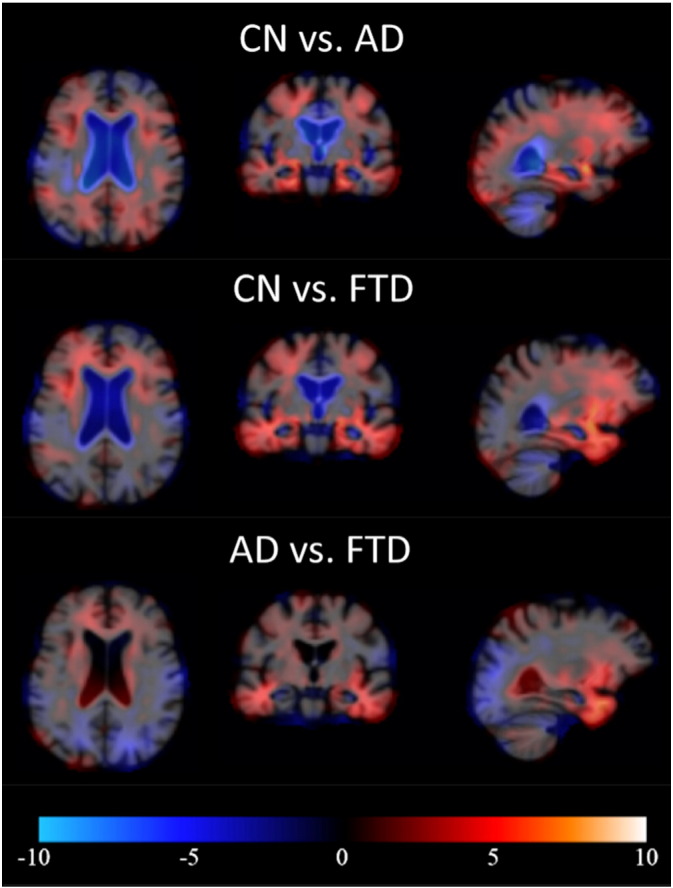
Fig. 4 — Examples of pair-wise t-maps for TBM. Red = smaller local volume in latter group, blue = larger local volume in latter group. (For interpretation of the references to color in this figure legend, the reader is referred to the web version of this article.)

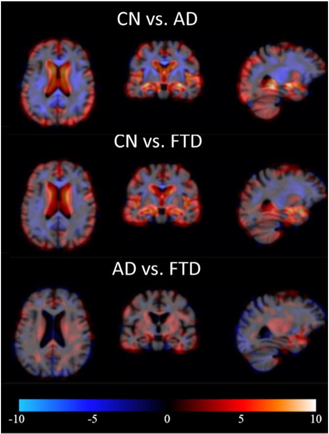
Fig. 5 — Examples of pair-wise t-maps for VBM. Red = smaller local GM concentration in latter group, blue = larger local GM concentration in latter group. (For interpretation of the references to color in this figure legend, the reader is referred to the web version of this article.)

Fig. 6 shows examples of correctly classified patients. The control subject shows well-preserved brain anatomy, whereas the AD patient has enlarged ventricles and medial temporal lobe atrophy. The FTD patient has large atrophy in the frontal and temporal lobes and enlarged ventricles. The VaD patient has vast regions of WMH that can be seen as bright regions in FLAIR image but also as hypointense regions in T1 image. The VaD patient has also notable brain atrophy, but the vascular findings dominate the DSI computation, and therefore the patient is classified as VaD.

Fig. 7 shows examples of the misclassified patients. The first case shows an AD patient that is classified as VaD because of the large WMH regions clearly visible in FLAIR image. The patients miss-classified as AD have typical brain atrophy patterns to AD, and the AD patient classified as FTD patient has atrophy also in frontal lobe.

The DSI values for each class are also presented in Fig. 6, Fig. 7. For the correctly classified patients in Fig. 6, the difference between the DSI of the correct class and the second highest DSI is large, indicating that the patient can be diagnosed with high likelihood to the first class. It can be seen that even for the most obvious DLB patients the difference to the other classes is quite small, indicating that the diagnosis to DLB cannot be done with high confidence using only imaging data. These results demonstrate the usability of the continuous indices that describe the likelihood of each type of dementia and, therefore, provide information to support clinical decision making. For example, for 50.4% of the patients the difference of the two largest DSI values is more than 0.06. For this subset of patients the classification accuracy is 80.7%, i.e., much higher than for the whole dataset (70.6%).

4. Discussion

In this paper, we performed an extensive study on differential diagnostics of dementias using only structural MRI data. A five-class classification (CN, AD, FTD, VaD, and DLB groups) was done using 10-fold cross-validation with a dataset of 504 patients. Several image quantification methods (volumetry, VBM, TBM, manifold learning, ROI-based grading, and vascular burden) were used to produce features for classification. The features were normalized to take into account age- and gender-related variation, and also the effect of MRI field strength was normalized. In addition, there was notable imbalance in the size of the study groups, which means that relatively high accuracy could have been obtained just by assigning all patients to the group with most patients. Therefore, in addition to the classification accuracy, the balanced accuracy was computed to adjust the results for the imbalance in the size of the study groups in the dataset.

A balanced classification accuracy of 69.1% was obtained when all the quantification methods were combined. In practice, it may not make sense to apply all quantification methods. The best combination of two quantification methods (ROI-based grading and vascular burden measure) gave already high balanced classification accuracy (67.7%) demonstrating that a well-chosen subset of quantification methods has the potential to differentiate accurately dementias. It is essential to include the vascular burden measure in the analysis, as it is needed to detect VaD patients. Otherwise, VBM, TBM, and/or ROI-based grading are reasonable choices to include in the analysis.

VaD patients could be detected with high sensitivity of 96%. Also controls (sensitivity 82%) and AD patients (sensitivity 74%) could be accurately classified. FTD patients were most often misclassified as AD patients (21% of FTD patients) because of the similar pattern of medial temporal lobe atrophy. The most difficult type of dementia to differentiate was DLB with sensitivity of 32% as there are no DLB specific structural or vascular changes.

The five-class classification was performed also using visual MRI ratings as classification features. The results were considerably worse (acc = 44.6%, Bacc = 51.6%) than the results for automatically determined features (acc = 70.6%, Bacc = 69.1%), which proves that the automatic methods are able to quantify more detailed information that is essential for the differentiation of the dementias.

Few studies have reported classification results for the differentiation of dementias (Barber et al., 1999, Varma et al., 2002, Klöppel et al., 2008, Ishii et al., 2007, Burton et al., 2009, Munoz-Ruiz et al., 2012). However, the comparison of different studies is very difficult, as the studied groups and the number of patients vary. Also, most of the studies have utilized only two-class classifications, whereas in this study we performed differential diagnosis with five classes.

The strength of this study was that the classification method utilized here provides a continuous index for each disease describing the likelihood that the patient has the particular disease. If the highest index value is much larger than the second largest index value, it is probable that the class given by the classifier is correct. If two or more diseases have indices close to each other, the clinician cannot rely much on the results. On the other hand, as mixed pathologies are very common (33.8% of all dementia patients (Holmes et al., 1999)), the indices might provide useful information for mixed diagnoses.

Numerous state of the art classification methods are able to perform multi-class classification. However, most of them, such as support vector machines, work as a black box approach, where, for example, the significance of individual features cannot be easily inferred. The key driver of the DSI concept has been the simplicity, i.e., to keep the mathematics behind classification simple and easy to understand but still provide high classification accuracy. This objective was kept in mind also when transforming the technology from two-class classification problems to multi-class classification.

Automated quantification methods and computerized decision support methods provide additional objective information for clinicians to support their diagnosis. This extra information might be especially useful for unexperienced clinicians that do not constantly meet patients with different dementias in daily practice. This will equalize the treatment of patients regardless of in which hospital they are diagnosed.

In this study, the clinical assessment based on MRI data, neuropsychological test results, clinical information, and occasionally cerebrospinal fluid data was regarded as the gold standard, which was used in the evaluation of automated MRI methods. The gold standard diagnoses were made in a standardized way and according to clinical criteria in a multidisciplinary consensus meetings. In order to perform the classification study, we only considered the core diagnosis and ignored all remarks about mixed pathologies. However, the situation is not as straightforward in clinical practice but mixed diagnoses are common, and the diagnosis of the dementia can be surely confirmed only in autopsy (Lopez et al., 2002, Rabinovici et al., 2008).

The imaging data used in this study was from a memory clinical cohort acquired during a period of about ten years. Consequently, image quality significantly varied. For example, data were acquired on 1.0 T, 1.5 T, and 3.0 T systems, while slice thickness of the FLAIR images varied between 1.0–6.5 mm. Using a more homogenous dataset could potentially improve results. However, the use of normal clinical imaging data shows that the proposed methods could be used in clinical practice where the data are often sub-optimal.

The quantification methods could be further developed. Asymmetry features might provide information for the discrimination of FTD from other groups. Also, a more comprehensive set of ROIs in manifold learning and ROI-based grading could improve the classification accuracy. The quantification of vascular characteristics could be further improved by including T2-weighted MR images in the analysis (Wang et al., 2012). In addition, functional imaging modalities, such as PET, SPECT, and fMRI, have proven to produce complementary information for the differential diagnostics of dementias (Jagust, 2006, Kantarci et al., 2012, Roman and Pascual, 2012, Varma et al., 2002, Duara et al., 1999), and diffusion weighted MRI can be used to quantify white matter damage (Zhang et al., 2009). These imaging methods could provide valuable additional data to the methodology presented in this paper.

Although in this paper we focused solely on imaging data, non-imaging data, such as the results of neuropsychological tests, CSF biomarkers and genetic data, are essential for the diagnostics of dementias, and no diagnosis should be done based on only imaging data. The objective of our further studies is to combine the methods studied in this paper with all the available non-imaging data in order to generate even more accurate classifier for the differential diagnostics of dementias.

This study was performed using imaging data from a single clinical center. In the future, our objective is to study how the methods presented can generalize for classifying patients from other clinical centers, and study if the data acquired from one center could be used to classify patients from another center.

5. Conclusions

In this paper, the differential diagnostics of the four most common neurodegenerative diseases causing dementia, AD, FTD, VaD, and DLB, and patients with SCD, which were regarded as the control subjects, was studied with a large dataset and multiple quantification methods using T1-weighted and FLAIR MR images. The results show that these diseases can be differentiated with a high accuracy of 70.6% using only imaging data. Different quantification methods provide complementary information, and consequently, the best results are obtained by utilizing several quantification methods. The results show that automatic quantification methods and computerized decision support methods are feasible for clinical practice and provide comprehensive information that may help clinicians in the near future.

Acknowledgements

This work has received funding from the European Union's Seventh Framework Programme for research, technological development and demonstration under grant agreements no. 611005 (PredictND) and no. 601055 (VPH-DARE@IT). The VUmc Alzheimer Center is supported by Alzheimer Nederland and Stichting VUmc fonds. The clinical database structure was developed with funding from Stichting Dioraphte.

Appendix A. Imaging parameters in each disease group

Table A.6, Table A.7, Table A.8, Table A.9

Table A.6.

Distributions of disease groups based on the MRI scanner. Also the classification accuracies and balanced accuracies are shown for the subsets of patients.

	Total	CN	AD	FTD	DLB	VaD	acc	Bacc
Siemens Impact 1.0 T	85	42	0	31	7	5	74.1	66.5
Siemens Sonata 1.5 T	66	12	37	9	6	2	65.2	64.1
GE Signa 1.5 T	28	2	15	6	4	1	60.7	56.3
GE Signa 3.0 T	317	61	170	41	30	15	71.9	70.2
Siemens Avanto 1.5 T	4	1	1	1	0	1	100.0	100.0
Philips Ingenuity 3.0 T	4	0	0	4	0	0	25.0	25.0

Open in a new tab

Table A.7.

Distributions of disease groups based on the field strength. Also the classification accuracies and balanced accuracies are shown for the subsets of patients.

	Total	CN	AD	FTD	DLB	VaD	acc	Bacc
1.0 T	85	42	0	31	7	5	74.1	66.5
1.5 T	98	15	53	16	10	4	65.3	65.6
3.0 T	321	16	170	45	30	15	71.3	69.4

Open in a new tab

Table A.8.

Distributions of disease groups based on the resolution of T1 images. Also the classification accuracies and balanced accuracies are shown for the subsets of patients.

	Total	CN	AD	FTD	DLB	VaD	acc	Bacc
high	488	177	214	89	44	24	71.1	69.0
low	16	1	9	3	3	0	56.3	41.7

Open in a new tab

Table A.9.

Distributions of disease groups based on the resolution of FLAIR images. Also the classification accuracies and balanced accuracies are shown for the subsets of patients.

	Total	CN	AD	FTD	DLB	VaD	acc	Bacc
high	348	58	199	44	29	18	71.8	68.2
low	156	60	24	48	18	6	68.0	67.7

Open in a new tab

show the distributions of the disease groups, and the classification and balance accuracies for different sub-sets of imaging data.

In total six MRI devices were used in this dataset (Table A.6), and most of the patients were analyzed with a 3.0 T device (Table A.7). None of the AD patients was scanned with the 1.0 T MRI device, and almost half of the patients with 1.0 T MRIs were CNs. This explains the high classification accuracy for the 1.0 T device. On the other hand, GE Signa 1.5 T was used mostly for the dementia patients. Consequently, the accuracy for this device is lower than for other devices. In general, 3.0 T devices seem to produce slightly better results than 1.5 T devices.

Because of the miss-balance in the distribution of the disease groups between the MRI devices, especially the lack of AD patients scanned with the 1.0 T device, there is a possibility that the results are biased. However, the normalization of the features as described in Section 2.5 should reduce the risk for the bias. Also, the classification accuracies for the patients with 3.0 T images (Table A.7) are very similar to the results for the whole dataset, which proves that such bias has not affected the studies significantly.

The images were also divided into two groups based on image resolution. The images that have the largest voxel dimension smaller that 1.5 mm establish the high resolution group, whereas rest of the images are defined as low resolution images. Table A.8 presents the distributions of disease groups and classification accuracies for the T1 resolution groups. Similarly, Table A.9 shows the results for the FLAIR resolution groups. Most of the T1 images have high resolution. For the small group of low resolution images, the classification accuracies are notably lower than for the high resolution images. However, this may also be explained by the miss-balance of the disease groups. There is much more low resolution FLAIR images. However, the difference in classification results between the high and low resolution groups is not that large, which can be explained by the fact that the classifications are mostly done based on the features derived from T1 images.

Appendix B. Multi-class DSI classifier

The DSI classifier is based on the comparison of patient's feature values to the feature values of database patients with known diagnosis (Fig. B.8). Let us assume that the diagnosis needs to be done between two diseases, or disease states, called ‘state 0’ and ‘state 1’. Now, the patient data are compared to the database patients belonging to either ‘state 0’ or ‘state 1’. The comparison is done using the distributions of the feature values in both states, and it is evaluated to which distribution the patient feature better fits. If the feature value is on average smaller in the ‘state 1’, a fitness value is computed for each feature as

fitness (x_{f}) = \frac{R_{state 1} (x_{f})}{R_{state 1} (x_{f}) + L_{state 0} (x_{f})},

(B.1)

where x_f is the value of the fth feature for the patient, R_state1(x_f) is the right integral of probability density function for ‘state 1’ and L_state0(x_f) is the left integral of probability density function for ‘state 0’. If the patient feature value fits perfectly to the distribution of ‘state 1’ and does not fit at all to the distribution of ‘state 0’, the fitness value is one. On the other hand, a value of zero indicates a perfect fit with the ‘state 0’.

Fig. B.8 — Visualization of the computation of the fitness value. Upper figure shows the probability distributions for the state 0 and the state 1, and lower figure shows the curve for the fitness value. The data shown here are for the volume of right hippocampus where the state 0 is the CN group and the state 1 is the FTD group. The dashed line shows an example for a patient with the right hippocampus volume of 1750 mm³. This feature value fits better to the distribution of state 1 resulting in high fitness value.

In addition, the importance of the features in differentiating the two disease states is computed using the database data. In practice, this is computed from the sensitivity and specificity of using the feature to classify the database patients:

relevance (f) = sensitivity (f) + specificity (f) - 1 .

(B.2)

This value, ranging from zero to one, is called the relevance.

The fitness values of all the features are combined using weighted averaging with the relevance values as the weights:

DSI = \frac{\sum_{f} relevance (f) \cdot fitness (x_{f})}{\sum_{f} relevance (f)} .

(B.3)

This combination gives a disease state index, a value between zero and one, that describes the likelihood of the patient belonging to the ‘state 1’ when the alternative diagnosis would be ‘state 0’.

In multi-class classification, normal two-class classifications are performed between all the disease pairs. This gives a set of DSI values (in this study 20) that describe the likelihood of a patient having the disease i when the alternative diagnosis would be the disease j: DSI(i,j). From these pair-wise DSI values, the total DSI values for each disease is computed by averaging the DSI's of the disease pair analyses:

DSI (i) = \frac{1}{N_{c} - 1} \sum_{j = 1}^{N_{c}, j \neq i} DSI (i, j),

(B.4)

where N_c is the number of diseases groups. This value gives a likelihood index of patient having the disease i. When performing multi-class classification, the patient is assigned to the class with the highest DSI(i) value.

Appendix C. Balanced accuracies for all combinations of quantification methods

	5-class	CN	CN	CN	CN	AD	AD	AD	FTD	FTD	VaD
vs.	vs.	vs.	vs.	vs.	vs.	vs.	vs.	vs.	vs.
A	FTD	VaD	DLB	FTD	VaD	DLB	VaD	DLB	DLB
tbm	53.8^a	86.9	88.6	87.9^a	78.5	76.0	73.2^a	63.7	84.2^a	78.0	77.0^a
vbm	57.4^a	86.1	89.3	90.4^a	83.6	76.6	73.9^a	65.4	84.1^a	78.0	73.8^a
vol	50.7^a	75.5	82.5	81.9^a	74.1	70.9	74.6^a	63.9	84.1^a	71.0	75.7^a
vasc	36.2	60.8	53.6	95.8	38.0	55.8	91.7	59.0	95.7	52.7	94.7
ml	44.5^a	87.4	85.4	82.3^a	69.0	77.4	60.9^a	62.5	73.9^a	73.6	61.1^a
grading	51.5^a	91.1	88.5	84.9^a	74.7	82.5	68.4^a	71.2	80.3^a	80.6	60.0^a
tbm + vbm	60.4^a	87.4	88.9	93.7	83.4	79.1	77.4^a	67.6	92.0^a	78.0	80.1^a
tbm + vol	57.1^a	87.3	88.6	93.3^a	78.8	75.8	80.1^a	68.6	85.2^a	74.8	86.3^a
tbm + vasc	64.2	87.1	88.3	97.1	78.1	76.3	93.2	63.7	95.2	77.5	95.8
tbm + ml	55.1^a	88.4	89.1	87.5	78.1	77.8	73.2	65.6	86.9^a	78.5	79.1^a
tbm + grading	55.4^a	88.6	89.7	90.0^a	77.7	78.4	75.3	62.6	84.8^a	78.0	77.0^a
vbm + vol	60.0^a	87.4	91.3	92.9^a	84.1	76.2	77.4^a	68.6	88.9^a	80.1	81.1^a
vbm + vasc	67.0	85.7	88.9	97.1	84.3	76.6	94.1	65.8	95.2	78.0	95.8
vbm + ml	59.0^a	86.9	89.3	90.4^a	83.2	78.7	74.2^a	66.2	86.8^a	77.5	73.8^a
vbm + grading	59.3^a	87.6	89.7	89.9^a	83.2	77.5	74.4^a	66.8	86.8^a	76.9	74.8^a
vol + vasc	59.4	75.1	82.5	97.5	74.3	70.4	93.4	64.4	94.7	70.4	95.8
vol + ml	52.5^a	77.5	84.0	84.4^a	73.0	72.7	77.6^a	64.4	79.8^a	71.0	75.7^a
vol + grading	53.3^a	83.1	84.8	87.4^a	73.3	73.6	79.7^a	64.1	81.4^a	71.0	73.6^a
vasc + ml	60.0	87.9	85.4	97.1	70.1	78.3	93.9	63.4	95.2	72.5	95.8
vasc + grading	67.7	90.7	88.6	97.1	74.7	83.4	94.1	72.5	95.2	80.6	95.8
ml + grading	53.8^a	90.5	89.6	85.3^a	76.2	81.3	66.9^a	71.1	73.4^a	76.3	63.2^a
tbm + vbm + vol	62.1^a	89.0	90.2	93.3^a	83.6	77.8	79.7^a	66.7	89.9^a	78.5	80.1^a
tbm + vbm + vasc	67.5	87.5	88.6	97.1	84.1	79.5	93.9	67.6	95.2	78.0	95.8
tbm + vbm + ml	60.3^a	88.7	89.4	91.6^a	84.5	79.2	77.4^a	68.4	92.0^a	76.9	80.1^a
tbm + vbm + grading	61.1^a	88.3	89.8	93.7^a	84.1	79.6	77.4^a	69.7	92.0^a	78.0	80.1^a
tbm + vol + vasc	65.9	87.3	89.2	97.1	78.3	76.4	93.2	68.6	95.2	74.8	95.8
tbm + vol + ml	57.2^a	87.9	90.0	93.3^a	76.4	76.3	79.7^a	68.6	84.7^a	73.7	86.3^a
tbm + vol + grading	59.7^a	89.0	89.5	95.8^a	78.3	78.1	79.9^a	68.8	85.2	73.2	84.3^a
tbm + vasc + ml	65.3	88.2	88.3	97.1	77.3	78.4	93.2	65.6	95.2	77.5	95.8
tbm + vasc + grading	64.8	88.8	88.8	97.1	77.7	79.3	93.4	62.4	95.2	76.9	95.8
tbm + ml + grading	56.2^a	89.0	89.7	91.6^a	78.1	79.8	75.3^a	64.3	87.9^a	79.6	77.0^a
vbm + vol + vasc	68.1	86.6	90.4	97.1	84.7	77.1	94.1	69.3	95.2	78.0	95.8
vbm + vol + ml	61.1^a	87.6	91.3	92.9^a	83.2	77.1	77.6^a	68.8	91.5^a	79.1	79.0^a
vbm + vol + grading	61.6^a	89.2	90.8	92.9^a	82.8	76.4	77.6^a	70.1	90.9^a	79.6	79.0^a
vbm + vasc + ml	68.3	87.0	88.9	97.1	83.9	77.6	94.1	67.7	95.2	77.5	95.8
vbm + vasc + grading	68.9	87.4	89.7	97.1	84.3	77.5	94.1	68.4	95.2	76.9	95.8
vbm + ml + grading	59.9^a	87.6	88.8	89.9^a	84.3	78.6	74.4^a	69.2	86.8^a	76.4	74.8^a
vol + vasc + ml	61.7	78.2	84.2	97.1	74.1	73.2	93.4	64.0	95.2	69.9	95.8
vol + vasc + grading	62.0	82.5	85.9	97.1	74.3	74.1	93.4	65.5	95.2	71.0	95.8
vol + ml + grading	55.0^a	84.0	85.7	86.9^a	74.5	77.7	78.0^a	65.4	82.4^a	73.1	75.7^a
vasc + ml + grading	66.6	90.3	89.6	97.1	76.2	81.9	93.9	71.6	95.2	76.8	95.8
tbm + vbm + vol + vasc	68.6	88.6	89.9	97.1	84.3	78.7	93.7	67.0	95.2	77.5	95.8
tbm + vbm + vol + ml	62.2^a	89.0	90.6	93.3^a	83.6	78.9	79.7^a	66.7	92.0^a	78.5	80.1^a
tbm + vbm + vol + grading	62.6^a	89.0	90.6	93.3^a	83.2	79.5	79.7^a	67.8	89.9^a	78.5	80.1^a
tbm + vbm + vasc + ml	68.0	88.5	89.1	97.1	85.1	79.7	93.9	68.4	95.2	76.9	95.8
tbm + vbm + vasc + grading	68.7	88.3	89.5	97.1	84.7	80.5	93.9	69.7	95.2	78.0	95.8
tbm + vbm + ml + grading	61.0^a	89.0	89.8	93.7^a	83.6	79.3	77.4^a	69.5	92.0^a	78.0	80.1^a
tbm + vol + vasc + ml	66.2	87.7	90.1	97.1	75.6	77.0	93.2	68.8	95.2	75.3	95.8
tbm + vol + vasc + grading	66.2	88.8	89.7	97.1	78.6	79.2	93.2	68.8	95.2	73.7	95.8
tbm + vol + ml + grading	59.6^a	88.6	90.4	95.8^a	79.0	79.5	79.9^a	68.6	84.7^a	73.7	84.3^a
tbm + vasc + ml + grading	65.7	89.0	88.8	97.1	77.7	80.2	93.4	65.2	95.2	78.5	95.8
vbm + vol + vasc + ml	68.3	87.2	90.4	97.1	84.3	77.5	93.9	69.3	95.2	78.0	95.8
vbm + vol + vasc + grading	69.0	88.5	89.9	97.1	83.9	77.9	93.9	70.3	95.2	77.5	95.8
vbm + vol + ml + grading	62.1^a	88.5	91.2	92.9^a	83.9	77.9	77.6^a	69.9	91.5^a	78.0	79.0^a
vbm + vasc + ml + grading	69.0	87.6	88.8	97.1	85.3	78.3	94.1	69.9	95.2	76.4	95.8
vol + vasc + ml + grading	63.7	83.3	85.9	97.1	75.6	78.1	93.4	67.0	95.2	73.1	95.8
tbm + vbm + vol + vasc + ml	68.9	88.6	90.3	97.1	84.3	79.3	93.7	67.0	95.2	77.5	95.8
tbm + vbm + vol + vasc + grading	69.0	88.6	90.3	97.1	83.9	80.2	93.9	68.0	95.2	77.5	95.8
tbm + vbm + vol + ml + grading	62.7^a	89.0	90.6	93.3^a	83.6	79.4	79.7^a	67.8	92.0^a	78.5	80.1^a
tbm + vbm + vasc + ml + grading	68.8	89.0	89.5	97.1	84.7	80.0	93.9	69.5	95.2	78.0	95.8
tbm + vol + vasc + ml + grading	66.9	88.4	90.5	97.1	79.6	79.7	93.4	68.4	95.2	74.8	95.8
vbm + vol + vasc + ml + grading	69.2	88.1	90.3	97.1	84.5	77.5	93.9	70.3	95.2	76.9	95.8
tbm + vbm + vol + vasc + ml + grading	69.1	88.6	90.3	97.1	84.3	80.1	93.7	68.2	95.2	77.5	95.8

Open in a new tab

vol = Volumes.

vasc = Vascular burden measure.

ml = Manifold learning.

Grading = ROI-based grading.

All data used for the VaD patients in training set.

Appendix D. Balanced accuracies for best individual features

Comparison	Feature	Bacc
CN vs. AD	Grading for CN, hippocampus region	89.7
Grading for AD, hippocampus region	88.7
VBM, Global	85.2
VBM, left cerebral white matter	82.7
TBM, left hippocampus	82.1
Grading for CN, frontal region	82.0
VBM, right cerebral white matter	81.1
VBM, right hippocampus	81.1
TBM, global	80.6
Manifold learning feature 3, hippocampus region	80.4
CN vs. FTD	VBM, global	89.1
Grading for CN, frontal region	85.4
TBM, global	84.6
VBM, left cerebral white matter	84.6
VBM, left anterior insula	83.1
Grading for CN, hippocampus region	82.5
VBM, right cerebral white matter	81.6
TBM, left hippocampus	81.3
Volumes, left anterior insula	80.8
TBM, left entorhinal area	80.4
CN vs. VaD	Vascular burden measure	95.8
CN vs. DLB	VBM, global	80.3
VBM, right cerebral white matter	79.4
VBM, left cerebral white matter	76.9
Grading for CN, hippocampus region	73.5
Grading for CN, frontal region	71.8
TBM, Right Caudate	71.6
VBM, Left Planum Polare	71.6
VBM, Left Caudate	70.5
VBM, Right Caudate	69.6
VBM, Left Planum Temporale	69.2
AD vs. FTD	Grading for AD, hippocampus region	77.1
Grading for FTD, frontal region	76.3
VBM, global	75.2
TBM, global	74.3
Grading for FTD, hippocampus region	73.8
TBM, left temporal pole	73.0
Volumes, left temporal pole	72.7
VBM, left temporal pole	72.5
VBM, left cerebral white matter	72.2
Manifold learning feature 7, hippocampus region	69.8
AD vs. VaD	Vascular burden measure	91.7
AD vs. DLB	Grading for CN, hippocampus region	72.7
Grading for AD, hippocampus region	71.7
Volumes, right entorhinal area	70.1
TBM, left caudate	69.5
VBM, left hippocampus	69.1
VBM, right hippocampus	67.7
VBM, right lateral ventricle	67.1
VBM, right amygdala	67.1
TBM, right amygdala	66.8
VBM, right inferior lateral ventricle	65.7
FTD vs. VaD	Vascular burden measure	95.7
FTD vs. DLB	Grading for FTD, frontal region	76.9
TBM, global	76.4
VBM, left lateral ventricle	75.8
VBM, right basal forebrain	75.8
VBM, left anterior insula	74.8
Volumes, left temporal pole	74.8
VBM, global	73.7
Grading for CN, frontal region	73.7
VBM, left fusiform gyrus	73.7
VBM, right cerebral white matter	72.7
VaD vs. DLB	Vascular burden measure	94.7

Open in a new tab

References

Aljabar P., Heckemann R., Hammers A., Hajnal J., Rueckert D. Multi-atlas based segmentation of brain images: atlas selection and its effect on accuracy. NeuroImage. 2009;46(3):726–738. doi: 10.1016/j.neuroimage.2009.02.018. [DOI] [PubMed] [Google Scholar]
Artaechevarria X., Munoz-Barrutia A., de Solorzano C.O. Combination strategies in multi-atlas image segmentation: application to brain MR data. IEEE Trans. Med. Imaging. 2009;28(8):1266–1277. doi: 10.1109/TMI.2009.2014372. [DOI] [PubMed] [Google Scholar]
Ashburner J., Friston K. Voxel-based morphometry — the methods. NeuroImage. 2000;11(6):805–821. doi: 10.1006/nimg.2000.0582. [DOI] [PubMed] [Google Scholar]
Ashburner J., Hutton C., Frackowiak R., Johnsrude I., Price C., Friston K. Identifying global anatomical differences: deformation-based morphometry. Hum. Brain Mapp. 1998;6(5-6):348–357. doi: 10.1002/(SICI)1097-0193(1998)6:5/6<348::AID-HBM4>3.0.CO;2-P. [DOI] [PMC free article] [PubMed] [Google Scholar]
Ballmaier M., O'Brien J.T., Burton E.J., Thompson P.M., Rex D.E., Narr K.L., McKeith I.G., DeLuca H., Toga A.W. Comparing gray matter loss profiles between dementia with Lewy bodies and Alzheimer's disease using cortical pattern matching: diagnosis and gender effects. NeuroImage. 2004;23(1):325–335. doi: 10.1016/j.neuroimage.2004.04.026. [DOI] [PubMed] [Google Scholar]
Barber R., Ballard C., McKeith I., Gholkar A., O'Brien J. MRI volumetric study of dementia with Lewy bodies: a comparison with AD and vascular dementia. Neurology. 2000;54(6):1304–1309. doi: 10.1212/wnl.54.6.1304. [DOI] [PubMed] [Google Scholar]
Barber R., Gholkar A., Scheltens P., Ballard C., McKeith I., O'Brien J. Medial temporal lobe atrophy on MRI in dementia with Lewy bodies. Neurology. 1999;52(6):1153–1158. doi: 10.1212/wnl.52.6.1153. [DOI] [PubMed] [Google Scholar]
Barber R., McKeith I., Ballard C., O'Brien J. Volumetric MRI study of the caudate nucleus in patients with dementia with Lewy bodies, Alzheimer's disease, and vascular dementia. J. Neurol. Neurosurg. Psychiatry. 2002;72(3):406–407. doi: 10.1136/jnnp.72.3.406. [DOI] [PMC free article] [PubMed] [Google Scholar]
Belkin M., Niyogi P. Vol. 14. 2002. Laplacian eigenmaps and spectral techniques for embedding and clustering; pp. 585–591. (Advances in Neural Information Processing Systems 14). [Google Scholar]
Brodersen K., Ong C.S., Stephan K., Buhmann J. Pattern Recognition (ICPR), 2010 20th International Conference on. 2010. The balanced accuracy and its posterior distribution; pp. 3121–3124. [Google Scholar]
Burton E., Karas G., Paling S., Barber R., Williams E., Ballard C., McKeith I., Scheltens P., Barkhof F., O'Brien J. Patterns of cerebral atrophy in dementia with Lewy bodies using voxel-based morphometry. NeuroImage. 2002;17(2):618–630. [PubMed] [Google Scholar]
Burton E.J., Barber R., Mukaetova-Ladinska E.B., Robson J., Perry R.H., Jaros E., Kalaria R.N., O'Brien J.T. Medial temporal lobe atrophy on MRI differentiates Alzheimer's disease from dementia with lewy bodies and vascular cognitive impairment: a prospective study with pathological verification of diagnosis. Brain. 2009;132(1):195–203. doi: 10.1093/brain/awn298. [DOI] [PubMed] [Google Scholar]
Coupé P., Eskildsen S.F., Manjón J.V., Fonov V.S., Pruessner J.C., Allard M., Collins D.L. Scoring by nonlocal image patch estimator for early detection of Alzheimer's disease. NeuroImage Clin. 2012;1(1):141–152. doi: 10.1016/j.nicl.2012.10.002. [DOI] [PMC free article] [PubMed] [Google Scholar]
Duara R., Barker W., Luis C. Frontotemporal dementia and Alzheimer's disease: differential diagnosis. Dement. Geriatr. Cogn. Disord. 1999;10(1):37–42. doi: 10.1159/000051210. [DOI] [PubMed] [Google Scholar]
Dubois B., Feldman H.H., Jacova C., DeKosky S.T., Barberger-Gateau P., Cummings J., Delacourte A., Galasko D., Gauthier S., Jicha G., Meguro K., O'Brien J., Pasquier F., Robert P., Rossor M., Salloway S., Stern Y., Visser P.J., Scheltens P. Research criteria for the diagnosis of Alzheimer's disease: revising the NINCDS-ADRDA criteria. Lancet Neurol. 2007;6(8):734–746. doi: 10.1016/S1474-4422(07)70178-3. [DOI] [PubMed] [Google Scholar]
Falahati F., Westman E., Simmons A. Multivariate data analysis and machine learning in Alzheimer's disease with a focus on structural magnetic resonance imaging. J. Alzheimers Dis. 2014;41(3):685–708. doi: 10.3233/JAD-131928. [DOI] [PubMed] [Google Scholar]
Fazekas F., Chawluk J., Alavi A., Hurtig H., Zimmerman R. MR signal abnormalities at 1.5 t in Alzheimer's dementia and normal aging. AJR Am. J. Roentgenol. 1987;149(2):351–356. doi: 10.2214/ajr.149.2.351. [DOI] [PubMed] [Google Scholar]
Feldman H.H., Pirttila T., Dartigues J.F., Everitt B., Van Baelen B., Schwalen S., Kavanagh S. Treatment with galantamine and time to nursing home placement in Alzheimer's disease patients with and without cerebrovascular disease. Int. J. Geriatr. Psychiatry. 2009;24(5):479–488. doi: 10.1002/gps.2141. [DOI] [PubMed] [Google Scholar]
Folstein M.F., Folstein S.E., McHugh P.R. Mini-mental state: a practical method for grading the cognitive state of patients for the clinician. J. Psychiatr. Res. 1975;12(3):189–198. doi: 10.1016/0022-3956(75)90026-6. [DOI] [PubMed] [Google Scholar]
Frisoni G., Laakso M., Beltramello A., Geroldi C., Bianchetti A., Soininen H., Trabucchi M. Hippocampal and entorhinal cortex atrophy in frontotemporal dementia and Alzheimer's disease. Neurology. 1999;52(1):91–100. doi: 10.1212/wnl.52.1.91. [DOI] [PubMed] [Google Scholar]
Guerrero R., Wolz R., Rao A.W., Rueckert D. Manifold population modeling as a neuro-imaging biomarker: application to ADNI and ADNI-GO. NeuroImage. 2014;94C:275–286. doi: 10.1016/j.neuroimage.2014.03.036. [DOI] [PubMed] [Google Scholar]
Guimond A., Meunier J., Thirion J. Average brain models. a convergence study. Comput. Vis. Image Underst. 2000;7:192–210. [Google Scholar]
Heckemann R.A., Hajnal J.V., Aljabar P., Rueckert D., Hammers A. Automatic anatomical brain MRI segmentation combining label propagation and decision fusion. NeuroImage. 2006;33(1):115–126. doi: 10.1016/j.neuroimage.2006.05.061. [DOI] [PubMed] [Google Scholar]
Holmes C., Cairns N., Lantos P., Mann A. Validity of current clinical criteria for Alzheimer's disease, vascular dementia and dementia with Lewy bodies. Br. J. Psychiatry. 1999;174:45–50. doi: 10.1192/bjp.174.1.45. [DOI] [PubMed] [Google Scholar]
Ishii K., Soma T., Kono A.K., Sofue K., Miyamoto N., Yoshikawa T., Mori E., Murase K. Comparison of regional brain volume and glucose metabolism between patients with mild dementia with Lewy bodies and those with mild Alzheimer's disease. J. Nucl. Med. 2007;48(5):704–711. doi: 10.2967/jnumed.106.035691. [DOI] [PubMed] [Google Scholar]
Jagust W. Positron emission tomography and magnetic resonance imaging in the diagnosis and prediction of dementia. Alzheimers Dement. 2006;2(1):36–42. doi: 10.1016/j.jalz.2005.11.002. [DOI] [PubMed] [Google Scholar]
Kantarci K., Lowe V.J., Boeve B.F., Weigand S.D., Senjem M.L., Przybelski S.A., Dickson D.W., Parisi J.E., Knopman D.S., Smith G.E., Ferman T.J., Petersen R.C., Jack C.R., Jr. Multimodality imaging characteristics of dementia with Lewy bodies. Neurobiol. Aging. 2012;33(9):2091–2105. doi: 10.1016/j.neurobiolaging.2011.09.024. [DOI] [PMC free article] [PubMed] [Google Scholar]
Klöppel S., Stonnington C.M., Chu C., Draganski B., Scahill R.I., Rohrer J.D., Fox N.C., Jack C.R., Ashburner J., Frackowiak R.S.J. Automatic classification of MR scans in Alzheimer's disease. Brain. 2008;131(3):681–689. doi: 10.1093/brain/awm319. [DOI] [PMC free article] [PubMed] [Google Scholar]
Koikkalainen J., Lötjönen J., Thurfjell L., Rueckert D., Waldemar G., Soininen H. Multi-template tensor-based morphometry: application to analysis of Alzheimer's disease. NeuroImage. 2011;56(3):1134–1144. doi: 10.1016/j.neuroimage.2011.03.029. [DOI] [PMC free article] [PubMed] [Google Scholar]
Koikkalainen J., Pölönen H., Mattila J., van Gils M., Soininen H., Lötjönen J., for the Alzheimer's Disease Neuroimaging Initiative Improved classification of Alzheimer's disease data via removal of nuisance variability. PLoS ONE. 2012;7(2) doi: 10.1371/journal.pone.0031112. 02) [DOI] [PMC free article] [PubMed] [Google Scholar]
Laakso M.P., Frisoni G.B., Könönen M., Mikkonen M., Beltramello A., Geroldi C., Bianchetti A., Trabucchi M., Soininen H., Aronen H.J. Hippocampus and entorhinal cortex in frontotemporal dementia and Alzheimer's disease: a morphometric MRI study. Biol. Psychiatry. 2000;47(12):1056–1063. doi: 10.1016/s0006-3223(99)00306-6. [DOI] [PubMed] [Google Scholar]
Leemput K.V., Maes F., Vandermeulen D., Suetens P. Automated model-based tissue classification of MR images of the brain. IEEE Trans. Med. Imaging. 1999;18(10):897–908. doi: 10.1109/42.811270. [DOI] [PubMed] [Google Scholar]
Lopez O., Becker J., Kaufer D., Hamilton R., Sweet R., Klunk W., DeKosky S. Research evaluation and prospective diagnosis of dementia with Lewy bodies. Arch. Neurol. 2002;59(1):43–46. doi: 10.1001/archneur.59.1.43. [DOI] [PubMed] [Google Scholar]
Lötjönen J., Wolz R., Koikkalainen J., Julkunen V., Thurfjell L., Lundqvist R., Waldemar G., Soininen H., Rueckert D. Fast and robust extraction of hippocampus from MR images for diagnostics of Alzheimer's disease. NeuroImage. 2011;56(1):185–196. doi: 10.1016/j.neuroimage.2011.01.062. [DOI] [PMC free article] [PubMed] [Google Scholar]
Lötjönen J., Wolz R., Koikkalainen J., Thurfjell L., Waldemar G., Soininen H., Rueckert D. Fast and robust multi-atlas segmentation of brain magnetic resonance images. NeuroImage. 2010;49(3):2352–2365. doi: 10.1016/j.neuroimage.2009.10.026. [DOI] [PubMed] [Google Scholar]
Mattila J., Koikkalainen J., Virkki A., Simonsen A., van Gils M., Waldemar G., Soininen H., Lötjönen J. A disease state fingerprint for evaluation of Alzheimer's disease. J. Alzheimers Dis. 2011;27(1):163–176. doi: 10.3233/JAD-2011-110365. [DOI] [PubMed] [Google Scholar]
Mattila J., Koikkalainen J., Virkki A., van Gils M., Lötjönen J. Design and application of a generic clinical decision support system for multiscale data. IEEE Trans. Biomed. Eng. 2012;59(1):234–240. doi: 10.1109/TBME.2011.2170986. Jan) [DOI] [PMC free article] [PubMed] [Google Scholar]
McKeith I., Galasko D., Kosaka K., Perry E., Dickson D., Hansen L., Salmon D., Lowe J., Mirra S., Byrne E., Lennox G., Quinn N., Edwardson J., Ince P., Bergeron C., Burns A., Miller B., Lovestone S., Collerton D., Jansen E., Ballard C., de Vos R., Wilcock G., Jellinger K., Perry R. Consensus guidelines for the clinical and pathologic diagnosis of dementia with Lewy bodies (DLB): report of the consortium on DLB international workshop. Neurology. 1996;47(5):1113–1124. doi: 10.1212/wnl.47.5.1113. [DOI] [PubMed] [Google Scholar]
McKeith I.G., Dickson D.W., Lowe J., Emre M., O'Brien J.T., Feldman H., Cummings J., Duda J.E., Lippa C., Perry E.K., Aarsland D., Arai H., Ballard C.G., Boeve B., Burn D.J., Costa D., Del Ser T., Dubois B., Galasko D., Gauthier S., Goetz C.G., Gomez-Tortosa E., Halliday G., Hansen L.A., Hardy J., Iwatsubo T., Kalaria R.N., Kaufer D., Kenny R.A., Korczyn A., Kosaka K., Lee V., Lees A., Litvan I., Londos E., Lopez O.L., Minoshima S., Mizuno Y., Molina J.A., Mukaetova-Ladinska E.B., Pasquier F., Perry R.H., Schulz J.B., Trojanowski J.Q., Yamada M., for the Consortium on DLB Diagnosis and management of dementia with Lewy bodies. third report of DLB consortium. Neurology. 2005;65(12):1863–1872. doi: 10.1212/01.wnl.0000187889.17253.b1. [DOI] [PubMed] [Google Scholar]
McKhann G., Drachman D., Folstein M., Katzman R., Price D., Stadlan E.M. Clinical diagnosis of Alzheimer’s disease: report of the NINCDS-ADRDA work group under the auspices of department of health and human services task force on Alzheimer's disease. Neurology. 1984;34(7):939–1944. doi: 10.1212/wnl.34.7.939. [DOI] [PubMed] [Google Scholar]
McKhann G.M., Knopman D.S., Chertkow H., Hyman B.T., Jack C.R., Jr., Kawas C.H., Klunk W.E., Koroshetz W.J., Manly J.J., Mayeux R., Mohs R.C., Morris J.C., Rossor M.N., Scheltens P., Carrillo M.C., Thies B., Weintraub S., Phelps C.H. The diagnosis of dementia due to Alzheimer's disease: Recommendations from the National Institute on Aging-Alzheimer's Association workgroups on diagnostic guidelines for Alzheimer’s disease. Alzheimers Dement. 2011;7(3):263–269. doi: 10.1016/j.jalz.2011.03.005. [DOI] [PMC free article] [PubMed] [Google Scholar]
Meyer J.S., Huang J., Chowdhury M.H. MRI confirms mild cognitive impairments prodromal for Alzheimer's, vascular and Parkinson-Lewy body dementias. J. Neurol. Sci. 2007;257(1-2):97–104. doi: 10.1016/j.jns.2007.01.016. [DOI] [PubMed] [Google Scholar]
Munoz-Ruiz M.A., Hartikainen P., Koikkalainen J., Wolz R., Julkunen V., Niskanen E., Herukka S.-K., Kivipelto M., Vanninen R., Rueckert D., Liu Y., Lötjönen J., Soininen H. Structural MRI in frontotemporal dementia: comparisons between hippocampal volumetry, tensor-based morphometry and voxel-based morphometry. PLoS ONE. 2012;7(12) doi: 10.1371/journal.pone.0052531. (12) [DOI] [PMC free article] [PubMed] [Google Scholar]
Neary D., Snowden J.S., Gustafson L., Passant U., Stuss D., Black S., Freedman M., Kertesz A., Robert P.H., Albert M., Boone K., Miller B.L., Cummings J., Benson D.F. Frontotemporal lobar degeneration. a consensus on clinical diagnostics criteria. Neurology. 1998;51(6):1546–1554. doi: 10.1212/wnl.51.6.1546. [DOI] [PubMed] [Google Scholar]
Pasquier F., Leys D., Weerts J., Mounier-Vehier F., Barkhof F., Scheltens P. Inter- and intraobserver reproducibility of cerebral atrophy assessment on MRI scans with hemispheric infarcts. Eur. Neurol. 1996;36(5):268–272. doi: 10.1159/000117270. [DOI] [PubMed] [Google Scholar]
Rabinovici G., Seeley W., Kim E., Gorno-Tempini M., Rascovsky K., Pagliaro T., Allison S., Halabi C., Kramer J., Johnson J., Weiner M., Forman M., Trojanowski J., DeArmond S., Miller B., Rosen H. Distinct MRI atrophy patterns in autopsy-proven Alzheimer's disease and frontotemporal lobar degeneration. Am. J. Alzheimers Dis. Other Demen. 2008;22(6):474–488. doi: 10.1177/1533317507308779. [DOI] [PMC free article] [PubMed] [Google Scholar]
Rascovsky K., Hodges J.R., Knopman D., Mendez M.F., Kramer J.H., Neuhaus J., van Swieten J.C., Seelaar H., Dopper E.G.P., Onyike C.U., Hillis A.E., Josephs K.A., Boeve B.F., Kertesz A., Seeley W.W., Rankin K.P., Johnson J.K., Gorno-Tempini M.-L., Rosen H., Prioleau-Latham C.E., Lee A., Kipps C.M., Lillo P., Piguet O., Rohrer J.D., Rossor M.N., Warren J.D., Fox N.C., Galasko D., Salmon D.P., Black S.E., Mesulam M., Weintraub S., Dickerson B.C., Diehl-Schmid J., Pasquier F., Deramecourt V., Lebert F., Pijnenburg Y., Chow T.W., Manes F., Grafman J., Cappa S.F., Freedman M., Grossman M., Miller B.L. Sensitivity of revised diagnostic criteria for the behavioural variant of frontotemporal dementia. Brain. 2011;134(9):2456–2477. doi: 10.1093/brain/awr179. [DOI] [PMC free article] [PubMed] [Google Scholar]
Roman G., Pascual B. Contribution of neuroimaging to the diagnosis of Alzheimer's disease and vascular dementia. Arch. Med. Res. 2012;43(8):671–676. doi: 10.1016/j.arcmed.2012.10.018. [DOI] [PubMed] [Google Scholar]
Román G.C., Tatemichi T.K., Erkinjuntti T., Cummings J.L., Masdeu J.C., Garcia J.H., Amaducci L., Orgogozo J.-M., Brun A., Hofman A., Moody D.M., O'Brien M.D., Yamaguchi T., Grafman J., Drayer B.P., Bennett D.A., Fisher M., Ogata J., Kokmen E., Bermejo F., Wolf P.A., Gorelick P.B., Bick K.L., Pajeau A.K., Bell M.A., DeCarli C., Culebras A., Korczyn A.D., Bogousslavsky J., Hartmann A., Scheinberg P. Vascular dementia. Diagnostic criteria for research studies: report of the NINDS-AIREN International workshop. Neurology. 1993;43(2):250–260. doi: 10.1212/wnl.43.2.250. [DOI] [PubMed] [Google Scholar]
Scheltens P., Launer L.J., Barkhof F., Weinstein H., van Gool W. Visual assessment of medial temporal lobe atrophy on magnetic resonance imaging: interobserver reliability. J. Neurol. 1995;242(9):557–560. doi: 10.1007/BF00868807. [DOI] [PubMed] [Google Scholar]
Siemers E.R., Sundell K.L., Carlson C., Case M., Sethuraman G., Liu-Seifert H., Dowsett S.A., Pontecorvo M.J., Dean R.A., Demattos R. Phase 3 solanezumab trials: secondary outcomes in mild Alzheimer's disease patients. Alzheimers Dement. 2015 doi: 10.1016/j.jalz.2015.06.1893. [DOI] [PubMed] [Google Scholar]
Studholme C., Hill D., Hawkes D. An overlap invariant entropy measure of 3d medical image alignment. Pattern Recogn. 1999;32(1):71–86. [Google Scholar]
Tong T., Wolz R., Coupé P., Hajnal J.V., Rueckert D. Segmentation of MR images via discriminative dictionary learning and sparse coding: application to hippocampus labeling. NeuroImage. 2013;76:11–23. doi: 10.1016/j.neuroimage.2013.02.069. [DOI] [PubMed] [Google Scholar]
Tustison N., Avants B., Cook P., Zheng Y., Egan A., Yushkevich P., Gee J. N4itk: improved N3 bias correction. IEEE Trans. Med. Imaging. 2010;29(6):1310–1320. doi: 10.1109/TMI.2010.2046908. June) [DOI] [PMC free article] [PubMed] [Google Scholar]
van der Flier W.M., Pijnenburg Y.A.L., Prins N., Lemstra A.W., Bouwman F.H., Teunissen C.E., van Berckel B.N.M., Stam C.J., Barkhof F., Visser P.J., van Egmond E., Scheltens P. Optimizing patient care and research: the Amsterdam dementia cohort. J. Alzheimers Dis. 2014;41(1):313–327. doi: 10.3233/JAD-132306. [DOI] [PubMed] [Google Scholar]
van Rikxoort E.M., Isgum I., Arzhaeva Y., Staring M., Klein S., Viergever M.A., Pluim J.P., van Ginneken B. Adaptive local multi-atlas segmentation: application to the heart and the caudate nucleus. Med. Image Anal. 2010;14(1):39–49. doi: 10.1016/j.media.2009.10.001. [DOI] [PubMed] [Google Scholar]
Varma A.R., Adams W., Lloyd J.J., Carson K.J., Snowden J.S., Testa H.J., Jackson A., Neary D. Diagnostic patterns of regional atrophy on MRI and regional cerebral blood flow change on spect in young onset patients with Alzheimer's disease, frontotemporal dementia and vascular dementia. Acta Neurol. Scand. 2002;105(4):261–269. doi: 10.1034/j.1600-0404.2002.1o148.x. [DOI] [PubMed] [Google Scholar]
Waldemar G., Dubois B., Emre M., Georges J., McKeith I.G., Rossor M., Scheltens P., Tariska P., Winblad B. Recommendations for the diagnosis and management of Alzheimer's disease and other disorders associated with dementia: Efns guideline. Eur. J. Neurol. 2007;14(1):e1–e26. doi: 10.1111/j.1468-1331.2006.01605.x. [DOI] [PubMed] [Google Scholar]
Wang Y., Catindig J.A., Hilal S., Soon H.W., Ting E., Wong T.Y., Venketasubramanian N., Chen C., Qiu A. Multi-stage segmentation of white matter hyperintensity, cortical and lacunar infarcts. NeuroImage. 2012;60(4):2379–2388. doi: 10.1016/j.neuroimage.2012.02.034. [DOI] [PubMed] [Google Scholar]
Whitwell J.L., Weigand S.D., Shiung M.M., Boeve B.F., Ferman T.J., Smith G.E., Knopman D.S., Petersen R.C., Benarroch E.E., Josephs K.A., Jack C.R. Focal atrophy in dementia with Lewy bodies on MRI: a distinct pattern from Alzheimer's disease. Brain. 2007;130(3):708–719. doi: 10.1093/brain/awl388. [DOI] [PMC free article] [PubMed] [Google Scholar]
Wolz R., Julkunen V., Koikkalainen J., Niskanen E., Zhang D.P., Rueckert D., Soininen H., Lötjönen J., the Alzheimer’s Disease Neuroimaging Initiative Multi-method analysis of MRI images in early diagnostics of Alzheimer's disease. PLoS ONE. 2011;6(10) doi: 10.1371/journal.pone.0025446. (10) [DOI] [PMC free article] [PubMed] [Google Scholar]
Zhang Y., Schuff N., Du A.-T., Rosen H.J., Kramer J.H., Gorno-Tempini M.L., Miller B.L., Weiner M.W. White matter damage in frontotemporal dementia and Alzheimer's disease measured by diffusion MRI. Brain. 2009;132(9):2579–2592. doi: 10.1093/brain/awp071. [DOI] [PMC free article] [PubMed] [Google Scholar]

[bb0005] Aljabar P., Heckemann R., Hammers A., Hajnal J., Rueckert D. Multi-atlas based segmentation of brain images: atlas selection and its effect on accuracy. NeuroImage. 2009;46(3):726–738. doi: 10.1016/j.neuroimage.2009.02.018. [DOI] [PubMed] [Google Scholar]

[bb0010] Artaechevarria X., Munoz-Barrutia A., de Solorzano C.O. Combination strategies in multi-atlas image segmentation: application to brain MR data. IEEE Trans. Med. Imaging. 2009;28(8):1266–1277. doi: 10.1109/TMI.2009.2014372. [DOI] [PubMed] [Google Scholar]

[bb0015] Ashburner J., Friston K. Voxel-based morphometry — the methods. NeuroImage. 2000;11(6):805–821. doi: 10.1006/nimg.2000.0582. [DOI] [PubMed] [Google Scholar]

[bb0020] Ashburner J., Hutton C., Frackowiak R., Johnsrude I., Price C., Friston K. Identifying global anatomical differences: deformation-based morphometry. Hum. Brain Mapp. 1998;6(5-6):348–357. doi: 10.1002/(SICI)1097-0193(1998)6:5/6<348::AID-HBM4>3.0.CO;2-P. [DOI] [PMC free article] [PubMed] [Google Scholar]

[bb0025] Ballmaier M., O'Brien J.T., Burton E.J., Thompson P.M., Rex D.E., Narr K.L., McKeith I.G., DeLuca H., Toga A.W. Comparing gray matter loss profiles between dementia with Lewy bodies and Alzheimer's disease using cortical pattern matching: diagnosis and gender effects. NeuroImage. 2004;23(1):325–335. doi: 10.1016/j.neuroimage.2004.04.026. [DOI] [PubMed] [Google Scholar]

[bb0030] Barber R., Ballard C., McKeith I., Gholkar A., O'Brien J. MRI volumetric study of dementia with Lewy bodies: a comparison with AD and vascular dementia. Neurology. 2000;54(6):1304–1309. doi: 10.1212/wnl.54.6.1304. [DOI] [PubMed] [Google Scholar]

[bb0035] Barber R., Gholkar A., Scheltens P., Ballard C., McKeith I., O'Brien J. Medial temporal lobe atrophy on MRI in dementia with Lewy bodies. Neurology. 1999;52(6):1153–1158. doi: 10.1212/wnl.52.6.1153. [DOI] [PubMed] [Google Scholar]

[bb0040] Barber R., McKeith I., Ballard C., O'Brien J. Volumetric MRI study of the caudate nucleus in patients with dementia with Lewy bodies, Alzheimer's disease, and vascular dementia. J. Neurol. Neurosurg. Psychiatry. 2002;72(3):406–407. doi: 10.1136/jnnp.72.3.406. [DOI] [PMC free article] [PubMed] [Google Scholar]

[bb0045] Belkin M., Niyogi P. Vol. 14. 2002. Laplacian eigenmaps and spectral techniques for embedding and clustering; pp. 585–591. (Advances in Neural Information Processing Systems 14). [Google Scholar]

[bb0050] Brodersen K., Ong C.S., Stephan K., Buhmann J. Pattern Recognition (ICPR), 2010 20th International Conference on. 2010. The balanced accuracy and its posterior distribution; pp. 3121–3124. [Google Scholar]

[bb0055] Burton E., Karas G., Paling S., Barber R., Williams E., Ballard C., McKeith I., Scheltens P., Barkhof F., O'Brien J. Patterns of cerebral atrophy in dementia with Lewy bodies using voxel-based morphometry. NeuroImage. 2002;17(2):618–630. [PubMed] [Google Scholar]

[bb0060] Burton E.J., Barber R., Mukaetova-Ladinska E.B., Robson J., Perry R.H., Jaros E., Kalaria R.N., O'Brien J.T. Medial temporal lobe atrophy on MRI differentiates Alzheimer's disease from dementia with lewy bodies and vascular cognitive impairment: a prospective study with pathological verification of diagnosis. Brain. 2009;132(1):195–203. doi: 10.1093/brain/awn298. [DOI] [PubMed] [Google Scholar]

[bb0065] Coupé P., Eskildsen S.F., Manjón J.V., Fonov V.S., Pruessner J.C., Allard M., Collins D.L. Scoring by nonlocal image patch estimator for early detection of Alzheimer's disease. NeuroImage Clin. 2012;1(1):141–152. doi: 10.1016/j.nicl.2012.10.002. [DOI] [PMC free article] [PubMed] [Google Scholar]

[bb0070] Duara R., Barker W., Luis C. Frontotemporal dementia and Alzheimer's disease: differential diagnosis. Dement. Geriatr. Cogn. Disord. 1999;10(1):37–42. doi: 10.1159/000051210. [DOI] [PubMed] [Google Scholar]

[bb0075] Dubois B., Feldman H.H., Jacova C., DeKosky S.T., Barberger-Gateau P., Cummings J., Delacourte A., Galasko D., Gauthier S., Jicha G., Meguro K., O'Brien J., Pasquier F., Robert P., Rossor M., Salloway S., Stern Y., Visser P.J., Scheltens P. Research criteria for the diagnosis of Alzheimer's disease: revising the NINCDS-ADRDA criteria. Lancet Neurol. 2007;6(8):734–746. doi: 10.1016/S1474-4422(07)70178-3. [DOI] [PubMed] [Google Scholar]

[bb0080] Falahati F., Westman E., Simmons A. Multivariate data analysis and machine learning in Alzheimer's disease with a focus on structural magnetic resonance imaging. J. Alzheimers Dis. 2014;41(3):685–708. doi: 10.3233/JAD-131928. [DOI] [PubMed] [Google Scholar]

[bb0085] Fazekas F., Chawluk J., Alavi A., Hurtig H., Zimmerman R. MR signal abnormalities at 1.5 t in Alzheimer's dementia and normal aging. AJR Am. J. Roentgenol. 1987;149(2):351–356. doi: 10.2214/ajr.149.2.351. [DOI] [PubMed] [Google Scholar]

[bb0090] Feldman H.H., Pirttila T., Dartigues J.F., Everitt B., Van Baelen B., Schwalen S., Kavanagh S. Treatment with galantamine and time to nursing home placement in Alzheimer's disease patients with and without cerebrovascular disease. Int. J. Geriatr. Psychiatry. 2009;24(5):479–488. doi: 10.1002/gps.2141. [DOI] [PubMed] [Google Scholar]

[bb0095] Folstein M.F., Folstein S.E., McHugh P.R. Mini-mental state: a practical method for grading the cognitive state of patients for the clinician. J. Psychiatr. Res. 1975;12(3):189–198. doi: 10.1016/0022-3956(75)90026-6. [DOI] [PubMed] [Google Scholar]

[bb0100] Frisoni G., Laakso M., Beltramello A., Geroldi C., Bianchetti A., Soininen H., Trabucchi M. Hippocampal and entorhinal cortex atrophy in frontotemporal dementia and Alzheimer's disease. Neurology. 1999;52(1):91–100. doi: 10.1212/wnl.52.1.91. [DOI] [PubMed] [Google Scholar]

[bb0105] Guerrero R., Wolz R., Rao A.W., Rueckert D. Manifold population modeling as a neuro-imaging biomarker: application to ADNI and ADNI-GO. NeuroImage. 2014;94C:275–286. doi: 10.1016/j.neuroimage.2014.03.036. [DOI] [PubMed] [Google Scholar]

[bb0110] Guimond A., Meunier J., Thirion J. Average brain models. a convergence study. Comput. Vis. Image Underst. 2000;7:192–210. [Google Scholar]

[bb0115] Heckemann R.A., Hajnal J.V., Aljabar P., Rueckert D., Hammers A. Automatic anatomical brain MRI segmentation combining label propagation and decision fusion. NeuroImage. 2006;33(1):115–126. doi: 10.1016/j.neuroimage.2006.05.061. [DOI] [PubMed] [Google Scholar]

[bb0120] Holmes C., Cairns N., Lantos P., Mann A. Validity of current clinical criteria for Alzheimer's disease, vascular dementia and dementia with Lewy bodies. Br. J. Psychiatry. 1999;174:45–50. doi: 10.1192/bjp.174.1.45. [DOI] [PubMed] [Google Scholar]

[bb0125] Ishii K., Soma T., Kono A.K., Sofue K., Miyamoto N., Yoshikawa T., Mori E., Murase K. Comparison of regional brain volume and glucose metabolism between patients with mild dementia with Lewy bodies and those with mild Alzheimer's disease. J. Nucl. Med. 2007;48(5):704–711. doi: 10.2967/jnumed.106.035691. [DOI] [PubMed] [Google Scholar]

[bb0130] Jagust W. Positron emission tomography and magnetic resonance imaging in the diagnosis and prediction of dementia. Alzheimers Dement. 2006;2(1):36–42. doi: 10.1016/j.jalz.2005.11.002. [DOI] [PubMed] [Google Scholar]

[bb0135] Kantarci K., Lowe V.J., Boeve B.F., Weigand S.D., Senjem M.L., Przybelski S.A., Dickson D.W., Parisi J.E., Knopman D.S., Smith G.E., Ferman T.J., Petersen R.C., Jack C.R., Jr. Multimodality imaging characteristics of dementia with Lewy bodies. Neurobiol. Aging. 2012;33(9):2091–2105. doi: 10.1016/j.neurobiolaging.2011.09.024. [DOI] [PMC free article] [PubMed] [Google Scholar]

[bb0140] Klöppel S., Stonnington C.M., Chu C., Draganski B., Scahill R.I., Rohrer J.D., Fox N.C., Jack C.R., Ashburner J., Frackowiak R.S.J. Automatic classification of MR scans in Alzheimer's disease. Brain. 2008;131(3):681–689. doi: 10.1093/brain/awm319. [DOI] [PMC free article] [PubMed] [Google Scholar]

[bb0145] Koikkalainen J., Lötjönen J., Thurfjell L., Rueckert D., Waldemar G., Soininen H. Multi-template tensor-based morphometry: application to analysis of Alzheimer's disease. NeuroImage. 2011;56(3):1134–1144. doi: 10.1016/j.neuroimage.2011.03.029. [DOI] [PMC free article] [PubMed] [Google Scholar]

[bb0150] Koikkalainen J., Pölönen H., Mattila J., van Gils M., Soininen H., Lötjönen J., for the Alzheimer's Disease Neuroimaging Initiative Improved classification of Alzheimer's disease data via removal of nuisance variability. PLoS ONE. 2012;7(2) doi: 10.1371/journal.pone.0031112. 02) [DOI] [PMC free article] [PubMed] [Google Scholar]

[bb0155] Laakso M.P., Frisoni G.B., Könönen M., Mikkonen M., Beltramello A., Geroldi C., Bianchetti A., Trabucchi M., Soininen H., Aronen H.J. Hippocampus and entorhinal cortex in frontotemporal dementia and Alzheimer's disease: a morphometric MRI study. Biol. Psychiatry. 2000;47(12):1056–1063. doi: 10.1016/s0006-3223(99)00306-6. [DOI] [PubMed] [Google Scholar]

[bb0160] Leemput K.V., Maes F., Vandermeulen D., Suetens P. Automated model-based tissue classification of MR images of the brain. IEEE Trans. Med. Imaging. 1999;18(10):897–908. doi: 10.1109/42.811270. [DOI] [PubMed] [Google Scholar]

[bb0165] Lopez O., Becker J., Kaufer D., Hamilton R., Sweet R., Klunk W., DeKosky S. Research evaluation and prospective diagnosis of dementia with Lewy bodies. Arch. Neurol. 2002;59(1):43–46. doi: 10.1001/archneur.59.1.43. [DOI] [PubMed] [Google Scholar]

[bb0170] Lötjönen J., Wolz R., Koikkalainen J., Julkunen V., Thurfjell L., Lundqvist R., Waldemar G., Soininen H., Rueckert D. Fast and robust extraction of hippocampus from MR images for diagnostics of Alzheimer's disease. NeuroImage. 2011;56(1):185–196. doi: 10.1016/j.neuroimage.2011.01.062. [DOI] [PMC free article] [PubMed] [Google Scholar]

[bb0175] Lötjönen J., Wolz R., Koikkalainen J., Thurfjell L., Waldemar G., Soininen H., Rueckert D. Fast and robust multi-atlas segmentation of brain magnetic resonance images. NeuroImage. 2010;49(3):2352–2365. doi: 10.1016/j.neuroimage.2009.10.026. [DOI] [PubMed] [Google Scholar]

[bb0180] Mattila J., Koikkalainen J., Virkki A., Simonsen A., van Gils M., Waldemar G., Soininen H., Lötjönen J. A disease state fingerprint for evaluation of Alzheimer's disease. J. Alzheimers Dis. 2011;27(1):163–176. doi: 10.3233/JAD-2011-110365. [DOI] [PubMed] [Google Scholar]

[bb0185] Mattila J., Koikkalainen J., Virkki A., van Gils M., Lötjönen J. Design and application of a generic clinical decision support system for multiscale data. IEEE Trans. Biomed. Eng. 2012;59(1):234–240. doi: 10.1109/TBME.2011.2170986. Jan) [DOI] [PMC free article] [PubMed] [Google Scholar]

[bb0190] McKeith I., Galasko D., Kosaka K., Perry E., Dickson D., Hansen L., Salmon D., Lowe J., Mirra S., Byrne E., Lennox G., Quinn N., Edwardson J., Ince P., Bergeron C., Burns A., Miller B., Lovestone S., Collerton D., Jansen E., Ballard C., de Vos R., Wilcock G., Jellinger K., Perry R. Consensus guidelines for the clinical and pathologic diagnosis of dementia with Lewy bodies (DLB): report of the consortium on DLB international workshop. Neurology. 1996;47(5):1113–1124. doi: 10.1212/wnl.47.5.1113. [DOI] [PubMed] [Google Scholar]

[bb0195] McKeith I.G., Dickson D.W., Lowe J., Emre M., O'Brien J.T., Feldman H., Cummings J., Duda J.E., Lippa C., Perry E.K., Aarsland D., Arai H., Ballard C.G., Boeve B., Burn D.J., Costa D., Del Ser T., Dubois B., Galasko D., Gauthier S., Goetz C.G., Gomez-Tortosa E., Halliday G., Hansen L.A., Hardy J., Iwatsubo T., Kalaria R.N., Kaufer D., Kenny R.A., Korczyn A., Kosaka K., Lee V., Lees A., Litvan I., Londos E., Lopez O.L., Minoshima S., Mizuno Y., Molina J.A., Mukaetova-Ladinska E.B., Pasquier F., Perry R.H., Schulz J.B., Trojanowski J.Q., Yamada M., for the Consortium on DLB Diagnosis and management of dementia with Lewy bodies. third report of DLB consortium. Neurology. 2005;65(12):1863–1872. doi: 10.1212/01.wnl.0000187889.17253.b1. [DOI] [PubMed] [Google Scholar]

[bb0200] McKhann G., Drachman D., Folstein M., Katzman R., Price D., Stadlan E.M. Clinical diagnosis of Alzheimer’s disease: report of the NINCDS-ADRDA work group under the auspices of department of health and human services task force on Alzheimer's disease. Neurology. 1984;34(7):939–1944. doi: 10.1212/wnl.34.7.939. [DOI] [PubMed] [Google Scholar]

[bb0205] McKhann G.M., Knopman D.S., Chertkow H., Hyman B.T., Jack C.R., Jr., Kawas C.H., Klunk W.E., Koroshetz W.J., Manly J.J., Mayeux R., Mohs R.C., Morris J.C., Rossor M.N., Scheltens P., Carrillo M.C., Thies B., Weintraub S., Phelps C.H. The diagnosis of dementia due to Alzheimer's disease: Recommendations from the National Institute on Aging-Alzheimer's Association workgroups on diagnostic guidelines for Alzheimer’s disease. Alzheimers Dement. 2011;7(3):263–269. doi: 10.1016/j.jalz.2011.03.005. [DOI] [PMC free article] [PubMed] [Google Scholar]

[bb0210] Meyer J.S., Huang J., Chowdhury M.H. MRI confirms mild cognitive impairments prodromal for Alzheimer's, vascular and Parkinson-Lewy body dementias. J. Neurol. Sci. 2007;257(1-2):97–104. doi: 10.1016/j.jns.2007.01.016. [DOI] [PubMed] [Google Scholar]

[bb0215] Munoz-Ruiz M.A., Hartikainen P., Koikkalainen J., Wolz R., Julkunen V., Niskanen E., Herukka S.-K., Kivipelto M., Vanninen R., Rueckert D., Liu Y., Lötjönen J., Soininen H. Structural MRI in frontotemporal dementia: comparisons between hippocampal volumetry, tensor-based morphometry and voxel-based morphometry. PLoS ONE. 2012;7(12) doi: 10.1371/journal.pone.0052531. (12) [DOI] [PMC free article] [PubMed] [Google Scholar]

[bb0220] Neary D., Snowden J.S., Gustafson L., Passant U., Stuss D., Black S., Freedman M., Kertesz A., Robert P.H., Albert M., Boone K., Miller B.L., Cummings J., Benson D.F. Frontotemporal lobar degeneration. a consensus on clinical diagnostics criteria. Neurology. 1998;51(6):1546–1554. doi: 10.1212/wnl.51.6.1546. [DOI] [PubMed] [Google Scholar]

[bb0225] Pasquier F., Leys D., Weerts J., Mounier-Vehier F., Barkhof F., Scheltens P. Inter- and intraobserver reproducibility of cerebral atrophy assessment on MRI scans with hemispheric infarcts. Eur. Neurol. 1996;36(5):268–272. doi: 10.1159/000117270. [DOI] [PubMed] [Google Scholar]

[bb0230] Rabinovici G., Seeley W., Kim E., Gorno-Tempini M., Rascovsky K., Pagliaro T., Allison S., Halabi C., Kramer J., Johnson J., Weiner M., Forman M., Trojanowski J., DeArmond S., Miller B., Rosen H. Distinct MRI atrophy patterns in autopsy-proven Alzheimer's disease and frontotemporal lobar degeneration. Am. J. Alzheimers Dis. Other Demen. 2008;22(6):474–488. doi: 10.1177/1533317507308779. [DOI] [PMC free article] [PubMed] [Google Scholar]

[bb0235] Rascovsky K., Hodges J.R., Knopman D., Mendez M.F., Kramer J.H., Neuhaus J., van Swieten J.C., Seelaar H., Dopper E.G.P., Onyike C.U., Hillis A.E., Josephs K.A., Boeve B.F., Kertesz A., Seeley W.W., Rankin K.P., Johnson J.K., Gorno-Tempini M.-L., Rosen H., Prioleau-Latham C.E., Lee A., Kipps C.M., Lillo P., Piguet O., Rohrer J.D., Rossor M.N., Warren J.D., Fox N.C., Galasko D., Salmon D.P., Black S.E., Mesulam M., Weintraub S., Dickerson B.C., Diehl-Schmid J., Pasquier F., Deramecourt V., Lebert F., Pijnenburg Y., Chow T.W., Manes F., Grafman J., Cappa S.F., Freedman M., Grossman M., Miller B.L. Sensitivity of revised diagnostic criteria for the behavioural variant of frontotemporal dementia. Brain. 2011;134(9):2456–2477. doi: 10.1093/brain/awr179. [DOI] [PMC free article] [PubMed] [Google Scholar]

[bb0240] Roman G., Pascual B. Contribution of neuroimaging to the diagnosis of Alzheimer's disease and vascular dementia. Arch. Med. Res. 2012;43(8):671–676. doi: 10.1016/j.arcmed.2012.10.018. [DOI] [PubMed] [Google Scholar]

[bb0245] Román G.C., Tatemichi T.K., Erkinjuntti T., Cummings J.L., Masdeu J.C., Garcia J.H., Amaducci L., Orgogozo J.-M., Brun A., Hofman A., Moody D.M., O'Brien M.D., Yamaguchi T., Grafman J., Drayer B.P., Bennett D.A., Fisher M., Ogata J., Kokmen E., Bermejo F., Wolf P.A., Gorelick P.B., Bick K.L., Pajeau A.K., Bell M.A., DeCarli C., Culebras A., Korczyn A.D., Bogousslavsky J., Hartmann A., Scheinberg P. Vascular dementia. Diagnostic criteria for research studies: report of the NINDS-AIREN International workshop. Neurology. 1993;43(2):250–260. doi: 10.1212/wnl.43.2.250. [DOI] [PubMed] [Google Scholar]

[bb0250] Scheltens P., Launer L.J., Barkhof F., Weinstein H., van Gool W. Visual assessment of medial temporal lobe atrophy on magnetic resonance imaging: interobserver reliability. J. Neurol. 1995;242(9):557–560. doi: 10.1007/BF00868807. [DOI] [PubMed] [Google Scholar]

[bb0255] Siemers E.R., Sundell K.L., Carlson C., Case M., Sethuraman G., Liu-Seifert H., Dowsett S.A., Pontecorvo M.J., Dean R.A., Demattos R. Phase 3 solanezumab trials: secondary outcomes in mild Alzheimer's disease patients. Alzheimers Dement. 2015 doi: 10.1016/j.jalz.2015.06.1893. [DOI] [PubMed] [Google Scholar]

[bb0260] Studholme C., Hill D., Hawkes D. An overlap invariant entropy measure of 3d medical image alignment. Pattern Recogn. 1999;32(1):71–86. [Google Scholar]

[bb0265] Tong T., Wolz R., Coupé P., Hajnal J.V., Rueckert D. Segmentation of MR images via discriminative dictionary learning and sparse coding: application to hippocampus labeling. NeuroImage. 2013;76:11–23. doi: 10.1016/j.neuroimage.2013.02.069. [DOI] [PubMed] [Google Scholar]

[bb0270] Tustison N., Avants B., Cook P., Zheng Y., Egan A., Yushkevich P., Gee J. N4itk: improved N3 bias correction. IEEE Trans. Med. Imaging. 2010;29(6):1310–1320. doi: 10.1109/TMI.2010.2046908. June) [DOI] [PMC free article] [PubMed] [Google Scholar]

[bb0275] van der Flier W.M., Pijnenburg Y.A.L., Prins N., Lemstra A.W., Bouwman F.H., Teunissen C.E., van Berckel B.N.M., Stam C.J., Barkhof F., Visser P.J., van Egmond E., Scheltens P. Optimizing patient care and research: the Amsterdam dementia cohort. J. Alzheimers Dis. 2014;41(1):313–327. doi: 10.3233/JAD-132306. [DOI] [PubMed] [Google Scholar]

[bb0280] van Rikxoort E.M., Isgum I., Arzhaeva Y., Staring M., Klein S., Viergever M.A., Pluim J.P., van Ginneken B. Adaptive local multi-atlas segmentation: application to the heart and the caudate nucleus. Med. Image Anal. 2010;14(1):39–49. doi: 10.1016/j.media.2009.10.001. [DOI] [PubMed] [Google Scholar]

[bb0285] Varma A.R., Adams W., Lloyd J.J., Carson K.J., Snowden J.S., Testa H.J., Jackson A., Neary D. Diagnostic patterns of regional atrophy on MRI and regional cerebral blood flow change on spect in young onset patients with Alzheimer's disease, frontotemporal dementia and vascular dementia. Acta Neurol. Scand. 2002;105(4):261–269. doi: 10.1034/j.1600-0404.2002.1o148.x. [DOI] [PubMed] [Google Scholar]

[bb0290] Waldemar G., Dubois B., Emre M., Georges J., McKeith I.G., Rossor M., Scheltens P., Tariska P., Winblad B. Recommendations for the diagnosis and management of Alzheimer's disease and other disorders associated with dementia: Efns guideline. Eur. J. Neurol. 2007;14(1):e1–e26. doi: 10.1111/j.1468-1331.2006.01605.x. [DOI] [PubMed] [Google Scholar]

[bb0295] Wang Y., Catindig J.A., Hilal S., Soon H.W., Ting E., Wong T.Y., Venketasubramanian N., Chen C., Qiu A. Multi-stage segmentation of white matter hyperintensity, cortical and lacunar infarcts. NeuroImage. 2012;60(4):2379–2388. doi: 10.1016/j.neuroimage.2012.02.034. [DOI] [PubMed] [Google Scholar]

[bb0300] Whitwell J.L., Weigand S.D., Shiung M.M., Boeve B.F., Ferman T.J., Smith G.E., Knopman D.S., Petersen R.C., Benarroch E.E., Josephs K.A., Jack C.R. Focal atrophy in dementia with Lewy bodies on MRI: a distinct pattern from Alzheimer's disease. Brain. 2007;130(3):708–719. doi: 10.1093/brain/awl388. [DOI] [PMC free article] [PubMed] [Google Scholar]

[bb0305] Wolz R., Julkunen V., Koikkalainen J., Niskanen E., Zhang D.P., Rueckert D., Soininen H., Lötjönen J., the Alzheimer’s Disease Neuroimaging Initiative Multi-method analysis of MRI images in early diagnostics of Alzheimer's disease. PLoS ONE. 2011;6(10) doi: 10.1371/journal.pone.0025446. (10) [DOI] [PMC free article] [PubMed] [Google Scholar]

[bb0310] Zhang Y., Schuff N., Du A.-T., Rosen H.J., Kramer J.H., Gorno-Tempini M.L., Miller B.L., Weiner M.W. White matter damage in frontotemporal dementia and Alzheimer's disease measured by diffusion MRI. Brain. 2009;132(9):2579–2592. doi: 10.1093/brain/awp071. [DOI] [PMC free article] [PubMed] [Google Scholar]

	CN	AD	FTD	DLB	VaD		CN	AD	FTD	DLB	VaD
CN	77	8	0	28	5	CN	65%	7%	0%	24%	4%
AD	25	65	62	64	7	AD	11%	29%	28%	29%	3%
FTD	8	21	46	13	4	FTD	9%	23%	50%	14%	4%
DLB	9	13	3	20	2	DLB	19%	28%	6%	43%	4%
VaD	0	3	1	3	17	VaD	0%	13%	4%	13%	71%

	CN	AD	FTD	DLB	VaD		CN	AD	FTD	DLB	VaD
CN	97	10	2	9	0	CN	82%	8%	2%	8%	0%
AD	14	164	14	12	19	AD	6%	74%	6%	5%	9%
FTD	6	19	57	5	5	FTD	7%	21%	62%	5%	5%
DLB	8	18	4	15	2	DLB	17%	38%	9%	32%	4%
VaD	0	0	0	1	23	VaD	0%	0%	0%	4%	96%

	CN	AD	FTD	DLB	VaD		CN	AD	FTD	DLB	VaD
CN	77	8	0	28	5	CN	65%	7%	0%	24%	4%
AD	25	65	62	64	7	AD	11%	29%	28%	29%	3%
FTD	8	21	46	13	4	FTD	9%	23%	50%	14%	4%
DLB	9	13	3	20	2	DLB	19%	28%	6%	43%	4%
VaD	0	3	1	3	17	VaD	0%	13%	4%	13%	71%

	CN	AD	FTD	DLB	VaD		CN	AD	FTD	DLB	VaD
CN	97	10	2	9	0	CN	82%	8%	2%	8%	0%
AD	14	164	14	12	19	AD	6%	74%	6%	5%	9%
FTD	6	19	57	5	5	FTD	7%	21%	62%	5%	5%
DLB	8	18	4	15	2	DLB	17%	38%	9%	32%	4%
VaD	0	0	0	1	23	VaD	0%	0%	0%	4%	96%

PERMALINK

Differential diagnosis of neurodegenerative diseases using structural MRI data

Juha Koikkalainen

Hanneke Rhodius-Meester

Antti Tolonen

Frederik Barkhof

Betty Tijms

Afina W Lemstra

Tong Tong

Ricardo Guerrero

Andreas Schuh

Christian Ledig

Daniel Rueckert

Hilkka Soininen

Anne M Remes

Gunhild Waldemar

Steen Hasselbalch

Patrizia Mecocci

Wiesje van der Flier

Jyrki Lötjönen

Abstract

Graphical abstract

Highlights

1. Introduction

2. Material and methods

2.1. Patient groups

2.2. Imaging

2.3. Atlases and templates

2.4. Image quantification methods

2.4.1. Pre-processing

2.4.2. Multi-atlas segmentation

Fig. 1.

2.4.3. Voxel-based morphometry

2.4.4. Tensor-based morphometry

2.4.5. Manifold learning

Fig. 2.

2.4.6. ROI-based grading

2.4.7. Segmentation of white matter hyperintensities

Fig. 3.

2.4.8. Segmentation of cortical infacortical infarcts

2.4.9. Segmentation of lacunar infarcts

2.4.10. Vascular burden measure

2.5. Normalization of features

2.6. Classification

2.7. Evaluation

Table 1.

3. Results

3.1. Clinical data and visual MRI ratings

Table 2.

Table 3.

3.2. Automatic MRI Results

Table 4.

Table 5.

Fig. 4.

Fig. 5.

Fig. 6.

Fig. 7.

4. Discussion

5. Conclusions

Acknowledgements

Appendix A. Imaging parameters in each disease group

Table A.6.

Table A.7.

Table A.8.

Table A.9.

Appendix B. Multi-class DSI classifier

Fig. B.8.

Appendix C. Balanced accuracies for all combinations of quantification methods

Appendix D. Balanced accuracies for best individual features

References

ACTIONS

PERMALINK

RESOURCES

Similar articles

Cited by other articles

Links to NCBI Databases

	CN	AD	FTD	DLB	VaD		CN	AD	FTD	DLB	VaD
CN	77	8	0	28	5	CN	65%	7%	0%	24%	4%
AD	25	65	62	64	7	AD	11%	29%	28%	29%	3%
FTD	8	21	46	13	4	FTD	9%	23%	50%	14%	4%
DLB	9	13	3	20	2	DLB	19%	28%	6%	43%	4%
VaD	0	3	1	3	17	VaD	0%	13%	4%	13%	71%

	CN	AD	FTD	DLB	VaD		CN	AD	FTD	DLB	VaD
CN	97	10	2	9	0	CN	82%	8%	2%	8%	0%
AD	14	164	14	12	19	AD	6%	74%	6%	5%	9%
FTD	6	19	57	5	5	FTD	7%	21%	62%	5%	5%
DLB	8	18	4	15	2	DLB	17%	38%	9%	32%	4%
VaD	0	0	0	1	23	VaD	0%	0%	0%	4%	96%