The Population Tracking Model: A Simple, Scalable Statistical Model for Neural Population Data

Cian O'Donnell; J Tiago Gonç alves; Nick Whiteley; Carlos Portera-Cailliau; Terrence J Sejnowski

doi:10.1162/NECO_a_00910

. Author manuscript; available in PMC: 2017 Dec 3.

Published in final edited form as: Neural Comput. 2016 Nov 21;29(1):50–93. doi: 10.1162/NECO_a_00910

The Population Tracking Model: A Simple, Scalable Statistical Model for Neural Population Data

Cian O'Donnell ¹, J Tiago Gonç alves ², Nick Whiteley ³, Carlos Portera-Cailliau ⁴, Terrence J Sejnowski ⁵

PMCID: PMC5712479 NIHMSID: NIHMS922088 PMID: 27870612

Abstract

Our understanding of neural population coding has been limited by a lack of analysis methods to characterize spiking data from large populations. The biggest challenge comes from the fact that the number of possible network activity patterns scales exponentially with the number of neurons recorded (∼2^Neurons). Here we introduce a new statistical method for characterizing neural population activity that requires semi-independent fitting of only as many parameters as the square of the number of neurons, requiring drastically smaller data sets and minimal computation time. The model works by matching the population rate (the number of neurons synchronously active) and the probability that each individual neuron fires given the population rate. We found that this model can accurately fit synthetic data from up to 1000 neurons. We also found that the model could rapidly decode visual stimuli from neural population data from macaque primary visual cortex about 65 ms after stimulus onset. Finally, we used the model to estimate the entropy of neural population activity in developing mouse somatosensory cortex and, surprisingly, found that it first increases, and then decreases during development. This statistical model opens new options for interrogating neural population data and can bolster the use of modern large-scale in vivo Ca²⁺ and voltage imaging tools.

1 Introduction

Brains encode and process information as electrical activity over populations of their neurons (Churchland & Sejnowski, 1994; Averbeck, Latham, & Pouget, 2006). Although understanding the structure of this neural code has long been a central goal of neuroscience, historical progress has been impeded by limitations in recording techniques. Traditional extracellular recording electrodes allowed isolation of only one or a few neurons at a time (Stevenson & Kording, 2011). Given that the human brain has on the order of 10¹¹ neurons, the contribution of such small groups of neurons to brain processing is likely minimal. To get a more complete picture, we would instead like to simultaneously observe the activity of large populations of neurons. Although the ideal scenario—recording every neuron in the brain—is out of reach for now, recent developments in electrical and optical recording technologies have increased the typical size of population recording so that many laboratories now routinely record from hundreds or even thousands of neurons (Stevenson & Kording, 2011). The advent of these big neural data has introduced a new problem: how to analyze them.

The most commonly applied analysis to neural population data is to simply examine the activity properties of each neuron in turn, as if they were recorded in separate animals. However responses of nearby neurons to sensory stimuli are often significantly correlated, implying that neurons do not process information independently (Perkel, Gerstein, & Moore, 1967; Gerstein & Perkel, 1969, 1972; Singer, 1999; Cohen & Kohn, 2011). As a result, performing a cell-by-cell analysis amounts to throwing away potentially valuable information on the collective behavior of the recorded neurons. These correlations are important because they put strong functional constraints on neural coding (Zohary, Shadlen, & Newsome, 1994; Averbeck et al., 2006).

If we consider each neuron to have two spiking activity states, ON or OFF, then a population of N neurons as a whole can have 2^N possible ON/OFF patterns at any moment in time. The probability of seeing any particular one of these population activity patterns depends on the brain circuit examined, the stimuli the animal is subject to, and perhaps also the internal brain state of the animal. Neural correlations and sparse firing imply that the probabilities of some activity patterns are more likely than others. To help understand the neural code, we would like to be able to estimate the probability distribution across all 2^N patterns, P_true. For small N, the probability of each pattern can be estimated by simply counting each time it appears, then dividing by the total number of time points recorded However, since the number of possible patterns increases exponentially with N, this histogram method is experimentally intractable for populations larger than, say, 10 neurons. For example, 20 neurons would require fitting 2²⁰ ≈ 10⁶ parameters—one for each possible activity pattern. To accurately fit this model by counting patterns alone would require data recorded for many weeks or months. The problem gets worse for larger numbers of neurons: each additional neuron recorded requires a doubling in the recording time to reach the same level of statistical accuracy. This explosive scaling implies that we can never know the true distribution of pattern probabilities for a large number of neurons in a real brain.

This problem remained intractable until a seminal paper in 2006 demonstrated a possible solution:fitting a statistical model to the data that matches only some of the key low-order statistics, such as firing rates and pairwise correlations, and assume nothing else (Schneidman, Berry, Segev, & Bialek 2006). The hope was that these basic statistics are sufficient for the model to capture the majority of structure present in the real data so that P_model ≈ P_true Indeed early studies showed that such pairwise maximum entropy models could accurately capture activity pattern probabilities from recordings of 10 to 15 neurons in retina and cortex (Schneidman et al., 2006; Shlens et al., 2006; Tang et al., 2008; Yu, Huang, Singer, & Nikolić, 2008). Unfortunately, however, later studies found that the performance of these pairwise models was poor for larger populations and in different activity regimes (Ohiorhenuan et al., 2010; Ganmor, Segev, & Schneidman, 2011; Yu et al., 2011; Yeh et al., 2010), as predicted by theoretical work (Roudi, Nirenberg & Latham, 2009; Macke, Murray, & Latham, 2011). As a consequence, variants of the pairwise maximum entropy models have been proposed that include higher-order correlation terms (Ganmor et al., 2011; Tkacik et al., 2013, 2014), but these are difficult to fit for large N and are not readily nor-malizable. Alternative approaches have also been developed that appear to provide better matches to data (Amari, Nakahara, Wu, & Sakai, 2003 Pillow et al., 2008; Macke, Berens, Ecker, Tolias, & Bethge, 2009; Macke Opper, & Bethge, 2011; Köster, Sohl-Dickstein, Gray, & Olshausen, 2014; Okun et al., 2012; Park, Archer, Latimer, & Pillow, 2013; Okun et al., 2015; Schölvinck, Saleem, Benucci, Harris, & Carandini, 2015; Cui, Liu, McFarland, Pack, & Butts, 2016), but these suffer from similar shortcomings (see Table 1). We suggest the following criteria for an ideal statistical model for neural population data:

It should accurately capture the structure in real neural population data.
Its fitting procedure should scale well to large N, meaning that the model's parameters can be fit to data from large neural populations with a reasonable amount of data and computational resources.
Quantitative predictions can be made from the model after it is fit.

Table 1.

Comparison of Properties of Various Statistical Models of Neural Activity.

Model	References	Number of Parameters	Sampling Possible?	Fit for Large N?	Direct Estimates of Pattern Probabilities?	Low-Dimensional Model of Entire Distribution?
Pairwise maximum entropy	Schneidman et al. (2006); Shlens et al. (2006)	∼N²	Yes	Difficult	Difficult	No
K-pairwise maximum entropy	Tkacik et al. (2013, 2014)	∼N²	Yes	Difficult	Difficult	No
Spatiotemporal maximum entropy	Marre et al. (2009); Nasser et al. (2013)	∼RN²	Yes	Difficult	Difficult	No
Semi-restricted Boltzmann Machine	Koster et al. (2014)	∼N²	Yes	Difficult	Difficult	No
Reliable interaction model	Ganmor et al. (2011)	Data dependent	No	Yes	Approximate	No
Generalized linear models	Pillow et al. (2008)	∼DN²	Yes	Difficult	No	No
Dichotomized gaussian	Amari et al. (2003); Macke et al. (2009)	∼N²	Yes	Yes	No	No
Cascaded logistic	Park et al. (2013)	∼N²	Yes	Yes	Yes	No
Population coupling	Okun et al. (2012, 2015)	3N	Yes	Yes	No	No
Population tracking	This study	N²	Yes	Yes	Yes	Yes

Open in a new tab

Note: For the “Number of parameters” column, N indicates the number neurons considered, ∼ indicates “scales with,”D indicates the number of coefficients per interaction term, and R indicates the number of timepoints across which temporal correlations are considered.

No existing model meets all three of these demands (see Table 1). Here we propose a novel, simple statistical method that does: the population tracking model. The model is specified by only N² parameters: N to specify the distribution of number of neurons synchronously active and a further N² –N for the conditional probabilities that each individual neuron is ON given the population rate. Although no model with N² parameters can ever fully capture all 2^N pattern probabilities, we find that the population tracking model strikes a good balance of accuracy, tractability, and usefulness: by design, it matches key features of the data; its parameters can be easily fit for large N; it is normalizable, allowing expression of pattern probabilities in closed form; and, most surprising, it allows estimation of measures of the entire probability distribution, as we demonstrate for neural populations as large as N = 1000.

Section 2 of this letter is structured as follows. In section 2.1 we introduce the basic mathematical form of the model and fit it to spiking data from macaque visual cortex as an illustration. In sections 2.2 and 2.3, we cover how the model parameters can be estimated from data and how to sample synthetic data from the fitted model. In section 2.4 we show how a reduced 3N-parameter model of the entire 2^N-dimensional pattern probability distribution can be derived from the model parameters and how this reduced model can be used to estimate the population entropy, and the divergence between the model fits to two different data sets. In sections 2.5, 2.6, and 2.7 we show how the model's estimates for entropy and pattern probabilities converge as a function of neuron number and time samples available. Finally, in sections 2.8 and 2.9, we show how the method can help give novel biological insights by applying it to two data sets: first, we use the model to decode stimuli from the recorded electrophysiological spiking responses in macaque V1, and second, we analyze in vivo two-photon Ca²⁺ imaging data from mouse somatosensory cortex to explore how the entropy of neural population activity changes during development.

2 Results

2.1 Overview of the Statistical Model with Example Application to Data

We consider parallel recordings of the electrical activity of a population of N neurons. If the recordings are made using electrophysiology, then spike sorting methods can be used to extract the times of action potentials emitted by each neuron from the raw voltage waveforms (Quiroga, 2012). If the data are recorded using imaging methods—for example via a Ca²⁺-sensitive fluorophore—then electrical spike times or neural firing rates can often be approximately inferred (Pnevmatikakis et al., 2016; Rahmati, Kirmse, Marković, Holthoff, & Kiebel, 2016). Regardless of the way in which the data are collected, at any particular time in the recording some subset of these neurons may be active (ON), and the rest inactive (OFF). In the case of electrophysiologically recorded spike trains, the neurons considered ON might be those that emitted one or more spikes within a particular time bin Δt. For fluorescence imaging data, a suitable threshold in the ΔF(t)/F₀ signal may be chosen to split neurons into ON and OFF groups, perhaps after also binning the data in time. Once we have binarized the neural activity data in this way, each neuron's activity across time is reduced to a binary sequence of zeros and ones, where a zero represents silence and a one represents activity. For example, the ith neuron' activity in the population might be x_i = 0, 1, 0, 0, 0, 1, 1, 0, 1 … The length of the sequence T is simply the total number of time bins recorded. The brain might encode sensory information about the world in these patterns of neural population activity.

Next, we can next group the neural population data into a large N × T matrix M, where each row from i = 1:N corresponds to a different neuron and each column from j = 1:T corresponds to a different time point. At any particular time point (the jth column of M), we could in principle see any possible pattern of inactive and active neurons, written as a vector of zeros and ones {x}_j = [x_1j, x_2j, …, x_Nj]^T. In general, there will be 2^N possible patterns of population activity or combinations of zeros and ones. In any given experiment, each particular pattern must have some ground-truth probability of appearing P_true({x}), depending on the stimulus, animal's brain state, and so on. We would like to estimate this 2^N-dimensional probability distribution. However, since direct estimation is impossible, we instead fit the parameters of a simpler statistical model that implicitly specifies a different probability distribution over the patterns, P_model ({x}). The hope is that for typical neural data, P_model({x}) ≈ P_true({x}). In Figure 1, we schematize the procedure for building and using such a model.

Schematic diagram of the model building and utilization procedure. The neural circuit generates activity patterns sampled from some implicit distribution *P_true*, which are recorded by an experimentalist as data. We estimate certain statistics of these data to be used as parameters for the model. The model is a mathematical equation that specifies a probability distribution over all possible patterns *P_model*, whether or not each pattern was ever observed in the recorded data. We can then use the model for several applications: to sample synthetic activity patterns, directly estimate pattern probabilities, or build an even simpler model of the entire pattern probability distribution to estimate quantities such as the entropy.

The statistical model we propose for neural population data contains two sets of parameters that are fit in turn. The first set are the N free parameters needed to describe the population synchrony distribution: the probability distribution Pr(K = k) = p(k) for the number of neurons simultaneously active K, where $K = \sum_{i = 1}^{N} x_{i}$ . This distribution acts as a measure of the aggregate higher-order correlations in the population and so may contain information about the dynamical state of the network. For example, during network oscillations, neurons may be mostly either all ON or all OFF together, whereas if the network is in an asynchronous mode, the population distribution will be narrowly centered around the mean neuron firing probabilities.

The second set of free model parameters is the conditional probabilities that each individual neuron is ON, given the total number of neurons active in the population, p (x_i = 1|K). For shorthand, we write p(x_i |K) instead of p(x_i = 1|K) for the remainder of this letter. Since there are N + 1 possible values of K, and N neurons, there are N(N + 1) of these parameters. However, we know by definition that when K = 0 (all neurons are silent) and K = N (all neurons are active), then we must have p(x|K = 0) = 0 and p(x|K = N) = 1, respectively. Hence, we are left with only N(N – 1) free parameters. Different neurons tend to have different dependencies on the population count because of their heterogeneity in average firing rates (Buzsáki & Mizuseki, 2014) and because some neurons tend to be closely coupled to the activity of their surrounding population while others act independently (Okun et al., 2015). These two types of neurons have previously been termed choristers and soloists, respectively.

Once the N² total free parameters have been estimated from data (we discuss how this can be done below), we can construct the model. It gives the probability of seeing any possible activity pattern, even for patterns we have never observed, as

\begin{matrix} p ({x}) = \frac{p (k)}{a_{k}} (\prod_{i = 1}^{N} p {(x_{i} | k)}^{x_{i}} {[1 - p (x_{i} | k)]}^{1 - x_{i}}) & where & k = \sum_{i = 1}^{N} x_{i} \end{matrix},

(2.1)

where a_k is a normalizing constant defined as the sum of the probabilities of all $(\begin{matrix} N \\ k \end{matrix})$ patterns in the set S(k), where $\sum_{i = 1}^{N} x_{i} = k$ under a hypothetical model where neurons are conditionally independent:

a_{k} = \sum_{{x} \in S (k)} (\prod_{i = 1}^{N} p {(x_{i} | k)}^{x_{i}} {[1 - p (x_{i} | k)]}^{1 - x_{i}}) .

(2.2)

The model can be interpreted as follows. Given the estimated synchrony distribution p(k) and set of conditional probabilities p(x_i|K), we imagine a family of N – 1 probability distributions q_k({x}), k ∈ [1 : N – 1] where pattern probabilities are specified by the conditional independence models $q_{k} ({x}) = \prod_{i = 1}^{N} p {(x_{i} | k)}^{x_{i}} {[1 - p (x_{i} | k)]}^{1 - x_{i}}$ . Now, using this family of distributions, we construct one single distribution p({x}) by rejecting all pattern each q_k({x}) where $\sum_{i = 1}^{N} x_{i} \neq k$ , concatenating the remaining distributions (which cover mutually exclusive subsets of the pattern state space) renormalizing so that the pattern probabilities sum to one. This implies that for any given activity pattern {x}, p({x}) ∝ q_k({x}).

More intuitively, the model can be thought of as having two component levels. First is a high-level component that matches the distribution for the population rate. This component counts how many neurons are active ignoring the neural identities and treating all neurons as homogeneous The second, low-level, component accounts for some of the heterogeneity between neurons. It asks, given a certain number of active neurons in the population, what is then the conditional probability that each individual neuron is active? This component captures two features of the data: the differences in firing rates between neurons, which can vary over many orders of magnitude (Buzsáki & Mizuseki, 2014), and the relationship between a neuron' s activity and the aggregate activity of its neighbors (Okun et al., 2015). Both of these features can potentially have large effects on the pattern probability distribution.

In Figure 2, we fit this statistical model to electrophysiology spike data recorded from a population of 50 neurons in macaque V1 while the animal was presented with a drifting oriented grating visual stimulus. A section of the original spiking data during stimulus presentation is shown in Figure 2A (top), along with synthetically generated samples from the model fitted to these data, below it in red. By definition, the model matches the original data's population synchrony distribution and conditional probability that each neuron is active (see Figure 2B). In Figure 2C, we show the model's prediction for statistics of the data that it was not fitted to.

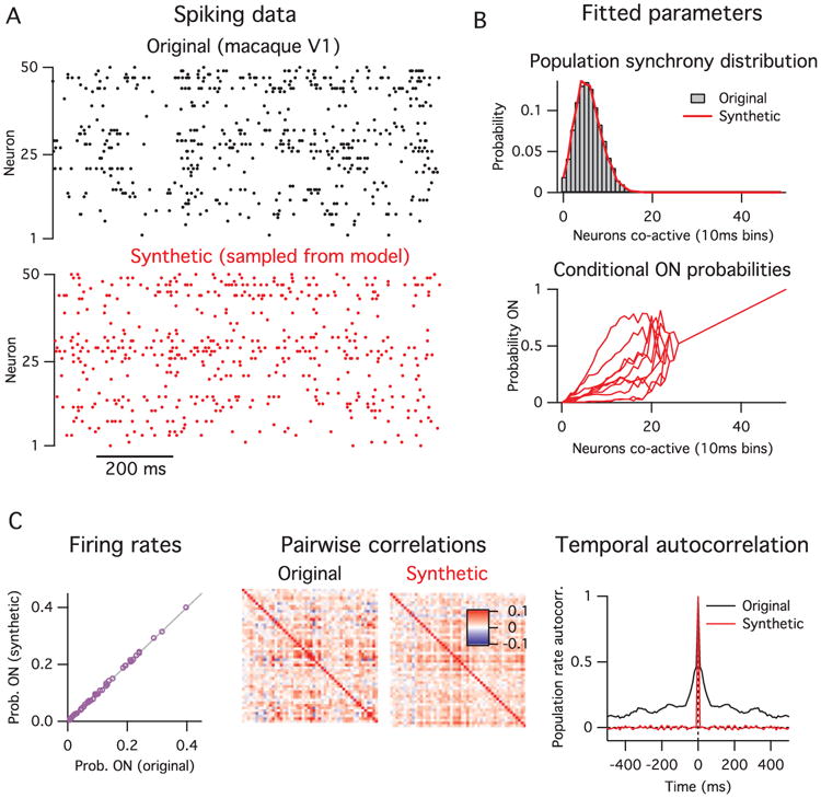
(A) Original spiking data (top, black) and synthetic data generated from model (bottom, red). (B) The model's fitted parameters. First, the population synchrony distribution (top), and, second, the conditional probability that each neuron is ON given the number of neurons active. The conditional ON probabilities of only 10 of the 50 neurons are shown for clarity. The curves converge to a straight line for k ķ 25 because those values of k were not observed in the data, so the parameter estimates collapse to the prior mean. (C) Comparison of other statistics of the data with the model's predictions. The model gives an exact match of the single neuron firing rates (left) and a partial match with the pairwise correlations (center), but does not match the data's temporal correlations (right).

In Figure 2C (left), the model almost exactly matches the average firing rate for each individual neuron. This is a direct consequence of the way the model is constructed and follows from the fits of the two sets of parameters. Hence, the model can capture the heterogeneity in neural firing rates.

Next, we compare the pairwise correlations between neurons from the original data with those from the data synthetically generated by sampling the model (see Figure 2C, center). Here we see only a partial match. Although the model captures the coarse features of the correlation matrix, it does not match the fine-scale structure on a pair-by-pair basis. For this example, the R² value between the model and data pairwise correlations was 0.52 (see Figure 10 in the appendix). In particular, the model accounts exactly for the population's mean pairwise correlation, because this is entirely due to the fluctuations in the population activity. We can demonstrate this effect directly by first subtracting away the covariance in the original data that can be accounted for by the model and then renormalizing to get a new correlation matrix (see Figure 10). Indeed this new correlation matrix is zero mean, but it retains much of the fine-scale structure between certain pairs of neurons. This implies that the model captures only coarse properties of the pairwise correlations.

The population tracking model partially recapitulates the pairwise correlation structure of the original data. In the left column are the pairwise correlation matrices from the example data shown in Figure 2 (top), for samples drawn from the population tracking model fit to these data (center), and the residual pairwise correlations in the data after subtracting the covariance accounted for by the population tracking model and renormalizing (bottom). In the center column are histograms of the pairwise correlations from each matrix in the left column. The scatter plots in the right column show the individual pairwise correlations of the model (red) and the data minus the model (purple) against the pairwise correlations in the original data. Note that the model almost exactly captures the mean pairwise correlation of the original data and part of the remaining structure (R² = 0.52).

Finally, the model does not at all match the temporal correlations present in the original data (see Figure 2C, right), since it assumes that each time bin is interchangeable. Note that this limitation is an ingredient of the model, not a failing per se. This property is shared with many other statistical methods commonly applied to neural population data (Schneidman et al., 2006; Macke et al., 2009; Cunningham & Yu, 2014; Okun et al., 2015).

These results show which statistics of the data that the population tracking model does and does not account for. Although other statistical models may more accurately account for pairwise or temporal correlation structure in the data, they typically do not scale well to large N (see Table 1). In the remainder of the letter we explore the model's behavior on large N data and show how we can take advantage of the particular form of the model to robustly estimate some high-level measures of the activity statistics, including the entropy of the data and the divergence between pairs of data sets. Since these measures are typically difficult or impossible to estimate using other common statistical models in the field, the population tracking model may allow experimenters to ask neurobiological questions that would be otherwise intractable.

2.2 Fitting the Model To Data

We now outline a procedure for fitting the statistical model's N² free parameters to neural population data. We assume that the data have already been preprocessed, as already discussed, and are in the format of either a binary N × T matrix M or a two-column integer list of active timepoints and their associated neuron IDs. We found that parameter fitting was fast; for example, fitting parameters to data from a 1 hour recording of 140 neurons was done on a standard desktop in about 1 minute.

2.2.1 Fitting the Population Activity Distribution

In the first set of parameters are the N values specifying the probability distribution for the number of neurons active p(k). In principle, K can take on any of the N + 1 values from 0 (the silent state) to N (the all ON state), but since we have the constraint that the probability distribution must normalize to one, one parameter can be calculated by default, so we need only fit N free parameters to fully specify the distribution. The most straightforward way to do this is by histogramming, which gives the maximum likelihood parameter estimates. We simply count how many neurons are ON at each of the T time points to get [K(t = 1), K(t = 2)… K(t = T)], then histogram this list and normalize to one so that our estimate p̂(k) = c_k/T, where c_k is the count of the number of time points where k neurons were active.

If the data statistics are sufficiently stationary relative to the timescale of recording, the error on each parameter individually scales ∼ 1/√T and independent of N. However, the relative error on each p̂(k) also scales $~ \sqrt{\frac{1 - p (k)}{p (k)}}$ , which implies large errors for rare values of K, when p(k) is small. Since neural activity is often sparse, we expect it to be quite common to observe small p(k) for large K, close to N (neurons are rarely all ON together). To avoid a case where we naively assign a probability of zero to a certain p(k) just because we never observe it in our finite data, we propose adding some form of regularization on the distribution p(k). A common method for regularization is to assume a prior distribution for p(k), then multiply it with the likelihood distribution from the data to compute the final posterior estimate for the parameters following Bayes' rule. If for convenience we assume a Dirichlet prior (conjugate to the multinomial distribution), then the posterior mean estimate for each parameter simplifies to

\hat{p} (k, α) = \frac{c_{k} + α}{T + N α},

where α is a small positive constant. This procedure is equivalent to adding the same small artificial count α to each empirical count c_k. For the examples presented in this study, we set α = 0.01.

2.2.2 Fitting the Conditional ON Probabilities for Each Neuron

The second step is to fit the N² – N unconstrained conditional probabilities that each neuron is ON given the total number of active neurons in the population, p(x|K). The simplest method to fit these parameters is by histogramming, similar to the above case for fitting the population activity distribution. In this case, we cycle through each value of K from 1 to N – 1, find the subset of time points at which there were exactly k neurons active, and count how many times each individual neuron was active at those time points, d_i,k. The maximum likelihood estimate for the conditional probability of the ith neuron being ON given k neurons in the population active is just p̂(x_i | k) = d_i,k/T_k, where T_k is the total number of time points where k neurons were active.

As before, given that some values of K are likely to be only rarely observed, we should also add some form of regularization to our estimates for p(x|K). We want to avoid erroneously assigning p(x_i |K) = 0, or any p(x_i |K) = 1 just because we had few data points available. Since x_i here is a Bernoulli variable, we regularize following standard Bayesian practice by setting a beta prior distribution over each p(x_i|K) because it is conjugate to the binomial distribution. Under this model, the posterior mean estimate for the parameters is

\hat{p} (x_{i} | k, β_{0}, β_{1}) = \frac{d_{i, k} + β_{1}}{β_{0} + β_{1} + T_{k}} .

Using the beta prior comes at the cost of setting its two hyperparameters, β₁ and β₂. We eliminate one of these free hyperparameters by constraining the prior's mean to be equal to k/N. This will pull the final parameter estimates toward the values that they would take if all neurons were homogeneous. The other free hyperparameter is the variance or width of the prior. This dictates how much the final parameter estimate should reflect the data: the wider the prior is, the closer the posterior estimate will be to the naive empirical data estimate. We found in practice good results if the variance of this prior scaled with the variance of the Bernoulli variables, ∝ μ(1 – μ) where μ = k/N. This guaranteed that the variance vanished as k became near 0 or N. For the examples presented in this study, we set the prior variance σ² = 0.5μ(1 – μ), and $β_{1} = \frac{μ}{σ^{2}} (μ - μ^{2} - σ^{2})$ and $β_{2} = β_{1} (\frac{1}{μ} - 1)$ .

An alternative method for fitting p(x|K) would be to perform logistic regression. Although in principle logistic regression should work well since we expect p(x|K) to typically be both monotonically increasing and correlated across neighboring values of k, we found in practice that as long as sufficient data were available, it gave inferior fits compared with the histogram method already discussed. However, for data sets with limited time samples, logistic regression might indeed be preferable. The other benefit would be that since logistic regression requires fitting of only two parameters per regression, if employed it would reduce the total number of the model's free parameters from N² to only 3N.

2.2.3 Calculating the Normalization Constants

The above expression for pattern probabilities includes a set of N – 1 constants A_k = {a₁, a₂…a_N–1} that are necessary to ensure that the distribution sums to one. These constants are not fit directly from data but instead follow from the parameters.

Each a_k is calculated separately for each value of k. They can be calculated in at least four ways. The most intuitive method is by the brute force enumeration of the probabilities of all $(\begin{matrix} N \\ k \end{matrix})$ possible patterns where k neurons are active, then summing the probabilities, as given by equation 2.2. Although this method is exact, it is computationally feasible only if $(\begin{matrix} N \\ k \end{matrix})$ is not too large, which can occur quite quickly when analyzing data from more than 20 to 30 neurons. The second method to estimate a_k is to draw N Bernoulli samples for many trials following the probabilities given by p(x|k), then count the fraction of trials in which the number of active neurons did in fact equal k. This method is approximate and inaccurate for large N because a_k → 0 as N → ∞.

The third method is to estimate a_k using importance sampling. We can rewrite equation 2.2 as

\begin{matrix} a_{k} = (\begin{matrix} N \\ k \end{matrix}) \frac{\sum_{{x} \in S (k)} (\prod_{i = 1}^{N} p {(x_{i} | k)}^{x_{i}} {[1 - p (x_{i} | k)]}^{1 - x_{i}})}{(\begin{matrix} N \\ k \end{matrix})} \\ = (\begin{matrix} N \\ k \end{matrix}) E [φ {x}], \end{matrix}

where {x} is a sample from the uniform distribution on S(k), and $φ ({x}) = (\prod_{i = 1}^{N} p {(x_{i} | k)}^{x_{i}} {[1 - p (x_{i} | k)]}^{1 - x_{i}})$ . If we have m such samples {x⁽¹⁾}, {x⁽²⁾}, …, {x^(m) }, then by the law of large numbers,

\frac{1}{m} \sum_{j = 1}^{m} φ ({x^{(j)}}) \to E [φ ({x})] = \frac{a_{k}}{(\begin{matrix} N \\ k \end{matrix})},

so by implication,

\sum_{j = 1}^{m} φ ({x^{(j)}}) \approx m E [φ ({x})] = \frac{a_{k} m}{(\begin{matrix} N \\ k \end{matrix})} .

If we fit a straight line in m to the partial sums $\hat{y} = \sum_{j = 1}^{m} φ ({x^{(j)}})$ by linear regression, say, ŷ = c₁m + c₀, we get

c_{1} m + c_{0} \approx \sum_{j = 1}^{m} φ ({x^{(j)}}) \approx \frac{a_{k} m}{(\begin{matrix} N \\ k \end{matrix})} .

Assuming that ŷ(m = 0) = 0, then the intercept c₀ = 0, so we are left with

c_{1} (\begin{matrix} N \\ k \end{matrix}) \approx a_{k} .

Finally, a fourth method follows from a procedure we present below for estimating a low-dimensional model of the entire pattern probability distribution as a sum of log normals.

2.2.4 The Implicit Prior on the Pattern Probability Distribution

By assuming a prior distribution over all of our parameters, we are implicitly assuming a prior distribution over the model's predicted pattern probabilities. What does that look like? For the population activity distribution, we have chosen a uniform value of α across all values of k, implying that our prior expects each level of population activity to be equally likely. The prior imposed on the second set of parameters, the p(x|K)s, would assign each neuron an identical conditional ON probability of k/N. Although the second set of priors is maximal entropy given the first set, it is important to note that the uniform prior over population activity is not maximum entropy, since each value of k carries a different number of patterns. Hence for large N, the prior will be concentrated on patterns where few (k near zero) or many (k near N) neurons are active.

A geometrical view of the effect of the priors can be given as follows. Since our N² parameters can each be written as a weighted linear sum of the 2^N pattern probabilities, they specify N² constraint hyperplanes for the solution in the 2^N-dimensional space of pattern probabilities. There are also other constraint hyperplanes that follow from constraints inherent to the problem, such as the fact that the pattern probabilities must sum to one and that p(x|K = 0) = 0. Since N² < 2^N (for all N > 4), an infinite number of solutions satisfy the constraints. Our final expression for the pattern probabilities is just a single point on the intersection of this set of hyperplanes. The effect of including priors on the parameters is to shift the hyperplanes so that our final solution is closer to prior pattern probabilities than that directly predicted by the data. In doing so, it ensures all patterns are assigned a nonzero probability of occurring, as any sensible model should.

2.3 Sampling from Model Given Parameters

Given the fitted parameters, sampling is straightforward using the following procedure:

Draw a sample for the integer number of neurons active k_sample from the range {0, …, N} according to the discrete distribution p(k). This can be done by drawing a random number from the uniform distribution and then mapping that value onto the inverse of the cumulative of p(k).
Draw N independent Bernoulli samples x = {x₁, x₂ … x_N}, one for each neuron, with the probability for the ith neuron given by p(x_i|k_sample). This is a candidate sample.
Count how many neurons are active in the candidate sample: $k_{sample}^{*} = \sum_{i = 1}^{N} x_{i}$ . If $k_{sample}^{*} = k_{sample}$ , accept the sample. If $k_{sample}^{*} \neq k_{sample}$ , reject the sample and return to step 2.

One benefit of this model is that since the sampling procedure is not iterative, sequential samples are completely uncorrelated.

2.4 Estimating the Full Pattern Probability Distribution, Entropy, and Divergence

2.4.1 Low-Dimensional Approximation to Pattern Probability Distribution

So far we have shown how to fit the model's parameters, calculate the probability of any specific population activity pattern, and sample from the model. Depending on the neurobiological question, an experimenter might also wish to use this model to calculate the probabilities of all possible activity patterns, either to examine the shape of the distribution or compute some measure that is a function of the entire distribution. One such measure, for example, is the joint population entropy H used in information-theoretic calculations, $H = - \sum_{i = 1}^{2^{N}} p ({x}_{i}) {log}_{2} p ({x}_{i}) .$

For small populations of neurons N ≾ 20, the probabilities of all 2^N possible activity patterns can be exhaustively enumerated. However, for larger populations, this brute force enumeration is not feasible due to limitations on computer storage space. For example, storing 2¹⁰⁰ ∼ 10³⁰ decimal numbers on a computer with 64-bit precision would require ∼ 10¹⁹ terabytes of storage space. Hence for most statistical models, such as classic pairwise maximum entropy models, this problem is either difficult or intractable (Broderick, Dudik, Tkacik, Schapire, & Bialek, 2007; although see Schaub & Schultz, 2012). Fortunately, the particular form of the model we propose implies that the distribution of pattern probabilities it predicts will, for sufficiently large k and N, tend toward the sum of a set of log-normal distributions, one for each value of k (see Figures 3B and 3C), as we explain below. Since the log-normal distribution is specified by only two parameters, we can fit this approximate model with only 3N parameters total, which can be readily stored for any reasonable value of N.

Calculating the distribution of population pattern probabilities and entropy for spiking data from macaque visual cortex. (A) Example raster plots of spiking data from 50 neurons in macaque V1 in response to static-oriented bar stimulus (left) and a blank screen (right). (B) The distribution of pattern probabilities for varying numbers of neurons is estimated for various values of the numbers of neurons active, k. (C) Summed total distribution of pattern probabilites for data recorded during stimulus (top, light blue) and blank screen (bottom, dark blue) conditions. The small bumps on top of the distributions are due to values of k that were unobserved in the data. Since the model assumes all patterns at these values are equally probable, they lead to the introduction of several sharp delta peaks to the pattern probability distribution. (D) The cumulative probability as a function of the cumulative number of patterns considered. Note that many-fold fewer activity patterns account for the bulk of the probability mass in the blank screen condition compared to during the stimulus. (E) Entropy per neuron of the pattern probability distribution for both conditions.

We derive the sum-of-log-normals distribution model as follows. First, we take the log of both sides of equation 2.1 to get

\begin{matrix} log p ({x}) = log p (k) + \sum_{i}^{N} log [p {(x_{i} | k)}^{x_{i}} {(1 - p (x_{i} | k))}^{(1 - x_{i})}] - log a_{k} \\ = log p (k) + \sum_{i}^{k} log [p (x_{i} | k) x_{i} \sum_{j}^{N - k} log (1 - p (x_{j} | k)) - log a_{k} \end{matrix},

(2.3)

where the second and third terms correspond to sums over the k active and (N – k) inactive neurons in {x}, respectively. Note that this equation is valid only for the cases where k ≥ 1. For clarity in what follows, we will temporarily represent p({x}) = θ and p({x}|k) = θ_k. Now let us consider the set L_k of the log probabilities for all $(\begin{matrix} N \\ k \end{matrix})$ patterns for a given level of population activity k, L_k = {log(p({x})}_k = {log(θ)}_k where $\sum_{i = 1}^{N} x_{i} = k$ . Since the population tracking model assumes that neurons are (pseudo) conditionally independent, then for sufficiently large N, according to the central limit theorem, the second and third terms in the sum in equation 2.3 will be normally distributed with some mean μ(k) and variance σ²(k), no matter what the actual distribution of p(x_i|K)'s is. Hence, if we were to histogram the log probabilities {log(θ)}_k of all patterns for a given k, their distribution could be approximated by the sum of two gaussians and two constants:

p {(log (θ))}_{k} \approx log p (k) + N (μ_{ON} (k), σ_{ON}^{2} (k)) + N (μ_{OFF} (k), σ_{OFF}^{2} (k)) - log a_{k} .

(2.4)

Note that this is a distribution over log pattern probabilities: it specifies the fraction of all neural population activity patterns that share a particular log probability of being observed.

The two normal distribution means are given by

\begin{matrix} μ_{ON} (k) = k 〈 log p (x | k) 〉, \\ μ_{OFF} (k) = (N - k) 〈 log (1 - p (x | k)) 〉, \end{matrix}

and the variances are

\begin{matrix} σ_{ON}^{2} (k) = k (\frac{N - k - 1}{N - 1}) var [log p (x | k)], \\ σ_{OFF}^{2} (k) = (N - k) (\frac{k - 1}{N - 1}) var [log (1 - p (x | k))], \end{matrix}

where the fractional terms in the variance equations are corrections because we are drawing without replacement from a finite population. Finally since we are adding two random variables (the second and third terms in equations 2.4), we also need to account for their covariance. Unfortunately, the value of this covariance depends on the data, and unlike the means and variances, we could find no simple formula to predict it directly from the parameters p(x|k). Hence, it should be estimated empirically by drawing random samples from the coupled distributions $N (μ_{ON} (k), σ_{ON}^{2} (k))$ and $N (μ_{OFF} (k), σ_{OFF}^{2} (k))$ and computing the covariance of the samples.

Although the log-normal approximation is valid when both K and N are large, the approximation will become worse when K is near 0 and N, no matter how large N is. This is problematic because neural data are often sparse, so small values of K are expected to be common and, hence, important to accurately model. Indeed, we found empirically that the distribution of log pattern probabilities at small K can become substantially skewed or, if the data come from neurons that include distinct subpopulations with different firing rates, even multimodal. We suggest that the experimenter examines the shape of the distribution by histogramming the probabilities of a large number of randomly chosen patterns to assess the appropriateness of the log-normal fit. The validity of the log-normal approximation can be formally assessed using, for example, the Lilliefors or Anderson-Darling tests. If the distribution is indeed non-log-normal for certain values of K, we suggest application of either or both of the following two ad hoc alternatives. First, for very small values of K (say, k ≾ 3), the number of patterns at this level of population synchrony $(\begin{matrix} N \\ k \end{matrix}) = \frac{N!}{k! (N - k)!}$ should also be small enough to permit brute force enumeration of all such pattern probabilities. Second, for slightly larger values of K (3 ≾ k ≾ 10), the distribution can be empirically fit by alternative low-dimensional parametric models, for example, a mixture-of-gaussians (MoG), which should be sufficiently flexible to capture any multimodality or skewness. In practice, we found that MoG model fits are typically improved by initializing the parameters with standard clustering algorithms, such as K-means.

One important precaution to take when fitting any parametric model to the pattern probability distributions (log normal, MoG, or otherwise) is to make sure that the resulting distributions are properly normalized so that the product of the integral of the approximated distribution of pattern probabilities for a given k, p(θ)_k, with the total number of possible patterns at that k, $(\begin{matrix} N \\ k \end{matrix})$ , does indeed equal the p(k) previously estimated from data:

(\begin{matrix} N \\ k \end{matrix}) \int_{0}^{1} p {(θ)}_{k} d θ = p (k) .

Although in principle this normalization should be automatic as part of the fitting procedure, even small errors in the distribution fit due to finite sampling can lead to appreciable errors in the normalization, due to the exponential sensitivity of the pattern probability sum on the fit in log coordinates. The natural place to absorb this correction is in the constant a_k, which in any case has to be estimated empirically so it will carry some error. Hence, we suggest that when performing this procedure, estimation of a_k should be left as the final step, when it can be calculated computationally as whatever value is necessary to satisfy the above normalization.

2.4.2 Calculating Population Entropy

Given the above reduced model of the pattern probability distribution, we could compute any desired function of the pattern probabilities (e.g., the mean or median pattern probability or the standard deviation). One example measure that is relevant for information theory calculations is Shannon's entropy, $H = - \sum_{i} p_{i} {log}_{2} p_{i}$ , measured in bits. This can be calculated by first decomposing the total entropy as

H = H_{k} + H (p ({x} | k)) = H_{k} + H {(θ)}_{k},

where $H_{k} = - \sum_{k = 0}^{N} p (k) {log}_{2} p (k)$ is the entropy of the population synchrony distribution and $H {(θ)}_{k} = \sum_{k = 0}^{N} p (k) H (θ_{k})$ is the conditional entropy of the pattern probability distribution given K. Given the sum-of-log-normals reduced model of the pattern probability distribution, the total entropy (in bits) of all patterns for a given k is

H (θ_{k}) = (\begin{matrix} N \\ k \end{matrix}) \int_{0}^{1} p {(θ)}_{k} \times [θ_{k} {log}_{2} θ_{k}] d θ .

This can be calculated by standard numerical integration methods separately for each possible value of K.

In the homogeneous case where all neurons are identical, all $(\begin{matrix} N \\ k \end{matrix})$ patterns for a given K will have equal probability of occurring, $p ({x}) | K = k) = p (k) / (\begin{matrix} N \\ k \end{matrix})$ . This situation maximizes the second term in the entropy expression and simplifies it to $H_{pop} = \sum_{k = 0}^{N} p (k) {log}_{2} \frac{(\begin{matrix} N \\ k \end{matrix})}{p (k)}$ .

To demonstrate these methods, we calculated the probability distribution across all 2⁵⁰ ≈ 10¹⁵ possible population activity patterns and the population entropy for an example spiking data set recorded from 50 neurons in macaque primary visual cortex. The presentation of a visual stimulus increases the firing rates of most neurons as compared to a blank screen (see Figure 3A). We found that this increase in firing rates leads to a shift in the distribution of pattern probabilities (see Figures 3C and 3D) and an increase in population entropy (see Figure 3E). Notably, a tiny fraction of all possible patterns accounts for almost all the probability mass. For the visually evoked data, around 10⁷ patterns accounted for 90% of the total probability, which implies that only $~ \frac{10^{7}}{10^{15}} = 0.000001 %$ of all possible patterns are routinely used. Although this result might not seem surprising given that neurons fire sparsely, any model that assumed independent neurons would likely overestimate this fraction because such a model would also overestimate the neural population's entropy (see below). These results demonstrate that the population tracking model can detect aspects of neural population firing that may be difficult to uncover with other methods.

2.4.3 Calculating the Divergence between Model Fits to Two Data Sets

Many experiments in neuroscience involve comparisons between neural responses under different conditions—for example, the firing rates of a neural population before and after application of a drug or the response to a sensory stimulus in the presence or absence of optogenetic stimulation. Therefore, it would be desirable to have a method for quantifying the differences in neural population pattern probabilities between two conditions. Commonly used measures for differences of this type are the Kullback-Leibler divergence and the related Jensen-Shannon divergence (Cover and Thomas, 2006; Berkes, Orbán, Lengyel, & Fiser, 2011). Calculation of either divergence involves a point-by-point comparison of the probabilities of each specific pattern under the two conditions. For small populations, this can be done by enumerating the probabilities of all possible patterns, but how would it work for large populations? On the face of it, the above approximate method for entropy calculation cannot help here, because that involved summarizing the distribution of pattern probabilities while losing the identities of individual patterns along the way. Fortunately, the form of the statistical model we propose does allow for an approximate calculation of the divergence between two pattern probability distributions, as follows. The Kullback-Leibler divergence from one probability distribution p(i) to another probability distribution q(i) is defined as

D_{KL} (p ‖ q) = \sum_{i} p (i) {log}_{2} \frac{p (i)}{q (i)} .

(2.5)

We can decompose this sum into N + 1 separate sums over the subsets of patterns with K neurons active:

D_{KL} (p ‖ q) = \sum_{k = 0}^{N} D_{KL} {(p ‖ q)}_{k} .

Hence, we just need a method to compute D_KL(p‖q)_k for any particular value of k. Notably, the term to be summed over in equation 2.5 can be seen as the product of two components, p(i) and ${log}_{2} \frac{p (i)}{q (i)}$ . In the preceding section, we showed that for sufficiently large k and N, the distribution of pattern probabilities at a fixed K is approximately log normal because of our assumption of conditional independence between neurons. Hence, the first component p(i) can be thought of as a continuous random variable that we will denote X₁, drawn from the log-normal distribution f(x₁). Because p(i) represents pattern probabilities, the range of f(x₁) is [0, 1]. The second component, ${log}_{2} \frac{p (i)}{q (i)}$ , in contrast, can be thought of as a continuous random variable that we will denote X₂, which is drawn from the normal distribution g(x₂), because by the same argument, $\frac{p (i)}{q (i)}$ is approximately log normally distributed, so its logarithm is normally distributed. Since this term is the logarithm of the ratio of two positive numbers, the range of g(x₂) is [−∞, ∞]. Now the term to be summed over can be thought of as the product of two continuous and dependent random variables Y = X₁X₂, with some distribution h(y).

Our estimate for the KL divergence $D_{KL}^{^}$ for a given k is, then, just the number of patterns at that value of k times the expected value of γ:

\begin{matrix} D_{KL}^{\land} {(p ‖ q)}_{k} = E [D_{KL} {(p ‖ q)}_{k}] = (\begin{matrix} N \\ k \end{matrix}) \int_{- \infty}^{\infty} y h (y) d y \\ = (\begin{matrix} N \\ k \end{matrix}) E [γ] \\ = (\begin{matrix} N \\ k \end{matrix}) E [X_{1} X_{2}] \\ = (\begin{matrix} N \\ k \end{matrix}) (E [X_{2}] E [X_{2}] + Cov [X_{1}, X_{2}]) \end{matrix} .

The three new terms in the last expression, 𝔼[X₁], 𝔼[X₂], and Cov[X1, X₂], can be estimated empirically by sampling a set of matched values of p({x}_i) and q({x}_i) from a large, randomly chosen subset of the $(\begin{matrix} N \\ k \end{matrix})$ patterns corresponding to a given value of k.

2.5 Model Fit Convergence for Large Numbers of Neurons

To test how the model scales with numbers of neurons and time samples, we fit it to synthetic neural population data from a different established statistical model, the dichotomized Gaussian (DG) (Macke et al., 2009). The DG model generates samples by thresholding a multivariate gaussian random variable in such a way that the resulting binary values match desired target mean ON probabilities and pairwise correlations. The DG is a particularly suitable model for neural data, because it has been shown that the higher-order correlations between “neurons” in this model reproduce many of the properties of high-order correlations seen in real neural populations recorded in vivo (Macke, Opper et al., 2011). This match may come from the fact that the thresholding behavior of the DG model mimics the spike threshold operation of real neurons.

For this section, we used the DG to simulate the activity of two equally sized populations of neurons, N₁ = N₂ = N/2: one population with a low firing rate of r₁ = 0.05 and the other with a higher firing rate of r₂ = 0.15. The correlations between all pairs of neurons were set at ρ = 0.1. We first estimated ground-truth pattern probability distributions by histogramming samples. Although there are 2^N possible patterns, the built-in symmetries in our chosen parameters meant that all patterns with the same number of neurons active from each group k₁ and k₂ share identical probabilities. Hence, the task amounted to estimating only the joint probabilities p(k₁, k₂) of the (N + 1)² configurations of having k₁ and k₂ neurons active. We generated as many time samples as were needed for this probability distribution to converge (T > 10⁹) for varying numbers of neurons ranging from N = 10 to N = 1000.

We then fit both our proposed model and several alternatives to further sets of samples from the DG, varying T from 100 to 1,000,000. Finally, we repeated the fitting procedure on many sets of fresh samples from the DG to examine variability in model fits across trials. To assess the quality of the fits, we use the population entropy as a summary statistic. We compared the entropy estimates of the population tracking model with five alternatives:

Independent neuron model. Neurons are independent, with individually fit mean firing rates estimated from the data. This model has N parameters.
Homogeneous population model. Neurons are identical but not independent. The model is constrained only by the population synchrony distribution p(k), as estimated from data. This model has N + 1 parameters.
Histogram. The probability of each population pattern is estimated by counting the number of times it appears and normalizing by T. This model has 2^N parameters.
Singleton entropy estimator (Berry, Tkacik, Dubuis, Marre, & da Silveira, 2013). This model uses the histogram method to estimate the probabilities of observed patterns in combination with an independent neuron model for the unobserved patterns. We implemented this method using our own Matlab code.
Archer-Park-Pillow (APP) method (Archer, Park, & Pillow, 2013). A Bayesian entropy estimator that combines the histogram method for observed patterns with a Dirichlet prior constrained by the population synchrony distribution. We implemented this method using the authors' publicly available Matlab code (http://github.com/pillowlab/CDMentropy).

We chose these models for comparison because they are tractable to implement. Although it is possible that other statistical approaches, such as the maximum entropy model family, would more accurately approximate the true data distribution, it is difficult to estimate the joint entropy from these models for data from 20 or more neurons (see Table 1).

In Figure 4 we plot the mean and standard deviation of the entropy/neuron estimates for this set of models as a function of the number of neurons (panels B and C) and number of time samples (panels D and E) analyzed. The key observation is that across most values of N and T, the majority of methods predict entropy values different from the true value (dashed line in all plots). These errors in the entropy estimates come from three sources: the finite sample variance, the finite sample bias, and the asymptotic bias.

Convergence of entropy estimate as a function of the number of neurons and time samples analyzed. (A) Example spiking data from the DG model with two subpopulations: a low firing rate group (filled black circles) and a higher firing rate group (open circles). Mean (B) and standard deviation (C) of estimated entropy per neuron as a function of the number of neurons analyzed, for each of the various models. The mean (D) and standard deviation (E) of estimated entropy per neuron as a function of the number of time steps considered, for data from varying numbers of neurons (left to right).

The finite sample variance is the variability in parameter estimates across trials from limited data, shown in Figures 4C and 4E as the standard deviation in entropy estimates. Notably, the finite sample variance decreases to near zero for all models within 10⁵ to 10⁶ time samples and is approximately independent of the number of neurons analyzed for the population tracking method (see Figures 4C and 4E).

The second error, the finite sample bias, arises from the fact that entropy is a concave function of p({x}). This bias is downward in the sense that the mean entropy estimate across finite data trials will always be less than the true entropy: 𝔼[H(p̂{x})] ≤ H(p({x})). Intuitively, any noise in the parameter estimates will tend to make the predicted pattern probability distribution lumpier than the true distribution, thus reducing the entropy estimate. Although this error becomes negligible for all models within a reasonable number of time samples for small numbers of neurons (N ≈ 10) (see Figures 4B and 4D), it introduces large errors for the histogram, singleton, and APP methods for larger populations. In contrast to the finite sample variance, the finite sample bias depends strongly on the number of neurons analyzed for all models, typically becoming worse for larger populations.

The third error, the asymptotic bias, is the error in entropy estimate that would persist even if infinite time samples were available. It is due to a mismatch between the form of the statistical model used to describe the data and the true underlying structures in the data. In Figure 4, this error is present for all models that do not include a histogram component: the independent, homogeneous population and population tracking models. Because the independent and homogeneous population models are maximum entropy given their parameters, their asymptotic bias in entropy will always be upward, meaning that these models will always overestimate the true entropy, given enough data. They are too simple to capture all of the structure in the data. Although the population tracking method may have either an upward or downward asymptotic bias, depending on the structure of the true pattern probability distribution, this error was small in magnitude for the example cases we examined.

The independent, homogeneous population and population tracking models converged to their asymptotic values within 10⁴–10⁵ time samples (see Figures 4D and 4E). The histogram, singleton, and APP methods, in contrast, performed well for small populations of neurons, N < 20, but strongly underestimated the entropy for larger populations (see Figures 4B, and 4D), even for T = 10⁶ samples.

The independent, homogeneous population, and population tracking models consistently predicted different values for the entropy. In order from greatest entropy to least entropy, they were: independent model, homogeneous population model, and population tracking. Elements of this ordering are expected from the form of the models. The independent model matches the firing rate of each neuron but assumes that they are uncorrelated, implying a high entropy estimate. Next, we found that the homogeneous population model had lower entropy than the independent model. However, this ordering will depend on the statistics of the data so may vary from experiment to experiment. The model we propose, the population tracking model, matches the data statistics of both the independent and the homogeneous population models. Hence, its predicted entropy must be less than or equal to both of these two previous models. One important note is that the relative accuracies of the various models should not be taken as fixed, but will depend on both the statistics of the data and the choices of the priors.

In summary, of the six models we tested on synthetic data, the population tracking model consistently performed best. It converged on entropy estimates close to the true value even for data from populations as large as 1000 neurons.

2.6 Population Tracking Model Accurately Predicts Probabilities for Both Seen and Unseen Patterns

The previous analysis involved estimating a single summary statistic, the entropy, for the entire 2^N-dimensional pattern probability distribution. But how well do the models do at predicting the probability of individual population activity patterns? To test this, we fit four of the six models to the same DG-generated data as the previous section, with N = 100 and T = 10⁶. As seen in Figures 4D and 4E, for data of this size, the entropy predictions of the three statistical models had converged, but the histogram method's estimate had not. We then drew 100 new samples from the same DG model, calculated all four models' predictions of pattern probability for each sample, and compared the predictions with the known true probabilities (see Figure 5).

Predicted pattern probabilities as a function of true pattern probabilities for a population of 100 neurons sampled from the same DG model as Figure 4. From left to right: independent model (blue), homogeneous population model (green), population tracking model (red), and histogram method (amber). In each plot, the darker-colored symbols correspond to patterns seen during model training and so were used in fitting the model parameters, and lighter-colored symbols correspond to new patterns that appeared only in the test set. The histogram plot (right) shows only data for the subset of patterns seen in both the training and test sets. Dashed diagonal line in each plot indicates identity.

The independent model's predictions deviated systematically from the true pattern probabilities. In particular, it tended to underestimate both high-probability and low-probability patterns, while overestimating intermediate probability patterns. It is important to note that the data in Figure 5 are presented on a log scale. Hence, these deviations correspond to many orders of magnitude error in pattern probability estimates. The homogeneous population model did not show any systematic biases in probability estimates but did show substantial scatter around the identity line, again implying large errors. This is to be expected since this model assumes that all patterns for a given k have equal probability. In contrast to these two models, the population tracking model that we propose accurately estimated pattern probabilities across the entire observed range. Finally, the histogram method failed dramatically. Although it predicted well the probabilities for the most likely patterns, it quickly deviated from the true values for rarer patterns. And worst of all, it predicts a probability of zero for patterns that it has not seen before, as evidenced by the large number of missing points in the right plot in Figure 5.

One final important point is that of the 100 test samples drawn from the DG model, 63 were not part of the training set (lighter-colored circles in Figure 5). However, the population tracking model showed no difference in accuracy for these unobserved patterns compared with the 37 patterns previously seen during training (darker circles in Figure 5). Together, these results show that the population tracking model can accurately estimate probabilities of both seen and unseen patterns for data from large numbers of neurons.

2.7 Model Performance for Populations with Heterogeneous Firing Rates and Correlations

In order to calculate the ground truth-pattern probabilities and entropy for large N for the above analysis, we assumed homogeneous firing rates and correlations to ensure symmetries in the pattern probability distributions. However, since the population tracking model also implicitly assumes some shared correlations across neurons due to their shared dependence on the population rate variable K, this situation may also bias the results in favor of the population tracking model in the sense that this may be the regime where P_model best matches P_true. Since in vivo neural correlations typically appear to have significant structure (see Figure 1C), we also examined the behavior of the model for a scenario with more heterogeneous firing rates and correlations. We repeated the above analysis using samples from the DG neuron model with N = 10, but with individual neuron firing rates drawn from a normal distribution μ = 0.1, σ = 0.02 and pairwise correlations drawn from a normal distribution with μ = 0.05, σ = 0.03 (see Figure 6A). We numerically calculated the 2¹⁰ = 1024 ground-truth pattern probabilities by exhaustively sampling from the DG model. We again varied the number of time samples from 100 to 1,000,000 and fit the population tracking model and several comparison models: the independent neuron model, the homogeneous population model, the histogram method, and also the pairwise maximum entropy model (Schneidman et al., 2006). We computed the Jensen-Shannon (JS) divergence, a measure of the difference between the true and model pattern probability distributions (see Figure 6B), entropy/neuron (see Figure 6C), and all 1024 individual pattern probabilities (see Figure 6D). Although the population tracking model outperformed the independent and homogeneous population models as before, it was outperformed by the pairwise maximum entropy model on this task. The JS divergence of the population tracking model saturated at a higher nonzero floor than the pairwise maximum entropy models in Figure 6B. However, the asymptotic error in the population tracking's estimate of entropy was minimal at +0.0015 bits, or 0.3% (see Figure 6C). It is difficult to ascertain whether the pairwise maximum entropy model would also outperform the population tracking model for large N and requires further study.

Performance of various models for data from 10 neurons with heterogeneous firing rates and correlations. (A) Example spiking data from the DG model (top left), with heterogeneous correlations and firing rates (bottom). Jensen-Shannon divergence of each model's predicted pattern probability distribution with the true distribution (B) and entropy per neuron (C) as a function of the number of time samples. (D) Predicted pattern probabilities versus true pattern probabilities for each of the tested models (left to right), for 1,000,000 time samples.

2.8 Decoding Neural Population Electrophysiological Data from Monkey Visual Cortex

We next tested the ability of the population tracking model to decode neural population responses to stimuli. We analyzed electrode array data recorded from anaesthetized macaque primary visual cortex in response to visual stimuli (see Figure 7A; see Zandvakili & Kohn, 2015, for details). Spike-sorting algorithms were applied to the raw voltage waveforms to extract the times of action potentials from multiunits. Altogether 131 different multiunits were recorded from a single animal. The animal was shown drifting oriented sinusoidal gratings chosen from eight orientations in a pseudorandom order. Each 1.28 s stimulus presentation was interleaved with a 1.5 s blank screen, and all eight possible stimulus orientations were presented 300 times each.

Decoding neural population spiking data from macaque primary visual cortex in response to oriented bar visual stimuli. (A) Example spiking data from 50 neurons during a single presentation of an oriented bar stimulus. Time zero indicates onset of stimulus. (B) Decoding performance as a function of time since stimulus onset for three different decoding models (different colored curves) and varying numbers of neurons (plots from left to right). Chance decoding level in all cases was 1/8 = 0.125. (C) The mean time since stimulus onset to reach 50% decoding accuracy for the independent (blue) and population tracking (red) models as a function of the number of neurons analyzed. The dashed curves indicate the time at which decoding accuracy first statistically exceeded noise levels. Time bin size fixed at 10 ms. The homogeneous population model is not shown because it never reached 50% decoding accuracy.

Our decoding analysis proceeded as follows. We first rebinned the data into 10 ms intervals. If a unit spiked one or more times in a time bin, it was labeled ON; otherwise it was labeled OFF. Second, we chose a random subset of N units from the 131 total and excluded data from the rest. Then, for a given stimulus orientation, we randomly split the data from the 300 trials into a 200-trial training set and a 100-trial test set. We concatenated the data from the 200 training trials and fit the population tracking model to this data set, along with two control statistical models: the independent model and the homogeneous population model. We repeated this procedure separately for the eight different stimulus orientations, so we were left with eight different sets of fitted parameters—one for each orientation. We then applied maximum likelihood decoding separately on neural responses to 100 randomly chosen stimuli from the test data set. Finally, we repeated the entire analysis 100 times for different random subsets of N neurons and training/test data set partitions and took a grand average of decoding performance.

We plot the decoding performance of the various statistical models as a function of time since the stimulus onset in Figure 7B. For all models, decoding was initially at chance level (1/8 = 0.125), then began to increase around 50 ms after stimulus onset, corresponding to the delay in spiking response in visual cortex (see Figure 7A). Decoding performance generally improved monotonically with both the number of neurons and number of time points analyzed for all models. However, decoding performance was much higher for the independent and population tracking models, which saturated at almost 100% correct, compared with about 25% correct for the homogeneous population model. Hence, for these data, it appears that the majority of information about the stimulus is encoded in the identities of which neurons are active, not in the total numbers of neurons active.

Although both the independent and population tracking models saturated to almost 100% decoding performance at long times, we found that for larger sets of neurons, the population tracking model's performance rose earlier in time than the independent neuron model (see Figures 7B and 7C). For 10 neurons, the independent model and population tracking model reached 50% accuracy at similar times after stimulus onset (146 ms with 95% CI [136.4:156] ms for the population tracking model and 142.5 ms with 95% CI [133.2:152.3] ms for the independent model). However, given spiking data from 100 neurons, the population tracking model reached 50% correct decoding performance at 66.1 ms after stimulus onset (95% CI [64.2:68] ms), whereas the independent model reached the same level later, at 76.2 ms after stimulus onset (95% CI [74.2:78] ms). Although superficially this may appear to be a modest difference in decoding speed, it is important to note that the baseline time for decoding above chance was not until 52.3 and 56.8 ms after stimulus onset for the population tracking and independent models, respectively. The reason for this late rise in decoding accuracy is the documented 50 ms lag in spiking response in macaque V1 relative to stimulus onset (Chen, Geisler, & Seidemann, 2006, 2008) (see Figure 7A). Given that we discretized the data into time bins of 10 ms, this implies that the population tracking model could decode stimuli mostly correctly given data from fewer than two time frames on average. In summary, these results show that the population tracking model can perform rapid stimulus decoding.

2.9 Entropy Estimation from Two-Photon Ca²⁺ Imaging Population Data from Mouse Somatosensory Cortex

As a second test case neuro-biological problem, we set out to quantify the typical number of activity patterns and entropy of populations of neurons in mouse neocortex across development. We applied our analysis method to spontaneous activity in neural populations from data previously recorded (Gonçalves, Anstey, Golshani, & Portera-Cailliau, 2013) by in vivo two-photon Ca²⁺ imaging in layer 2/3 primary somatosensory cortex of unanaesthetized wild-type mice with the fluorescent indicator Oregon green BAPTA-1. The original data were recorded at about 4 Hz (256 ms time frames), but for this analysis, we resampled the data into 1 s time bins because we found that it optimized a trade-off between catching more neurons in the active state versus maintaining a sufficient number of time frames for robust analysis.

To compare neural activity across development we used the Shannon entropy/neuron, h (see Figures 8H and 8I). Shannon entropy is a concept adopted from information theory that quantifies the uniformity of a probability distribution. If all patterns were equally probable, then h = 1 bit. At the opposite extreme, if only one pattern were possible, then h = 0 bits. It also has a functional interpretation as the upper limit on the amount of information the circuit can code (Cover & Thomas, 2006).

Entropy of neural populations in mouse somatosensory cortex increases and then decreases during development. (A) Example Ca²⁺ imaging movie from mice ages P9–11 (left), P14–16 (center), and P30–40 (right). (B) Mean ON probability of neurons by group. Each circle corresponds to the mean across all neurons recorded in a single animal; bars represent group means. (C) Probability density of the fraction of active neurons for sets of 50 neurons. Light gray traces are distributions from single animals; heavy black traces are group means. (D) Mean pairwise correlation between neurons in each group. (E) Cumulative distribution of pattern probabilities for each group, for sets of 50 neurons. Note log scale on x-axes. (F) Entropy per neuron as a function of the number of neurons analyzed. (G) Estimate of mean entropy per neuron for 100 neurons.

We performed the analysis on data from mice at three developmental age points: P9–11 (n = 13), P14–16 (n = 8), and P30–40 (n = 7). These correspond to time points just before (P9–11) and after (P14–P16), the critical period for cortical plasticity, and mature stage post-weaning (P30–P40). Entropy is determined by two main properties of the neural population activity: the activity levels of the neurons and their correlations. We found that mean ON probability increased between ages P9–P11 and P14–16 (p = 0.0016), then decreased again at age P30–40 (p = 0.0024). As previously observed (Rochefort et al., 2009; Golshani et al., 2009; Gonçalves et al., 2013), mean pairwise correlations decreased across development (p < 0.001, P9–11 versus P14–16) (see Figure 8D) so that as animals aged, there were fewer synchronous events when many neurons were active together (see Figures 8A and 8C).

What do these statistics predict for the distribution of activity patterns exhibited by neural circuits? Interestingly, activity levels and correlations are expected to have opposite effects on entropy: in the sparse firing regime, any increased ON probability should increase the entropy by increasing the typical number of activity patterns due to combinatorics, while an increase in correlations should decrease the entropy because groups of neurons will tend to be either all ON or all OFF together.

When we quantified the entropy of the pattern probability distributions, we found a nonmonotonic trajectory across development (see Figures 8F and 8G). For 100-neuron populations, in young animals at P9–11, we found a low group mean entropy of about 0.38 bits/neuron (CI [0.347:0.406]), followed by an increase at P14-16 (p < 0.001) to about 0.49 bits/neuron (CI [0.478:0.517]), and then a decrease in adulthood P30-P40 (p = 0.036) to about 0.45 bits/neuron (CI [0.418:0.476]). Although these shifts in dimensionality were subtle as estimated by entropy, they correspond to exponentially large shifts in pattern number. For example, 100-neuron populations in P14-16 animals showed an average of 5.6 × 10¹⁰ patterns, while 100-neuron populations in P30–40 animals showed an eight-fold fewer number of approximately 7.1 × 10⁹ typical patterns (data not shown). One interpretation of these findings is that young animals compress their neural representations of stimuli into a small dictionary of activity patterns, then expand their representations into a larger dictionary at P14–16, before again reducing the coding space again in adulthood, P30–40.

Is the shift in cortical neural population entropy across development due to changes in firing rates, correlations, or both? We assessed this by fitting two control models to the same Ca²⁺ imaging data: the independent neuron model and the homogeneous population model (see Figure 9). The independent neuron model captures changes in neural firing rates across development, including the heterogeneity in firing rates across the population, but inherently assumes that all correlations are fixed at zero. Although the independent model predicted a significant decrease in entropy between P14–P16 and P30-P40 (p = 0.014) similar to the population tracking model, it did not detect an increase in entropy from P9–P11 to P14–P16 (p = 0.13) (see Figure 9B, left).

Mouse somatosensory cortex entropy trajectories are not captured by either the independent or homogeneous population models. (A) Entropy per neuron estimated from the independent (blue circles) or homogeneous population (green) models against the same quantity estimated from the population tracking model, for data from mice of three age groups (left, center, and right plots). Each circle indicates the joint entropy estimated for 100-neuron population recording from a single animal. Note that the independent and homogeneous population models always estimate greater entropy values than the population tracking model. (B) Same data as panel A plotted to compare to Figure 8G. Note that neither the independent (blue, left) nor homogeneous population (green, right) models predict the inverted-U shaped trajectory uncovered by the population tracking model (see Figure 8G).

The homogeneous population model captures a different set of statistics. By matching the population synchrony distribution, it fits both the mean neuron firing rates and mean pairwise correlations. However, it also assumes that all neurons have identical firing rates and identical correlations; hence, it does not capture any of the population heterogeneity that the independent neuron model does. In contrast to the independent model, the homogeneous population model did predict the increase in entropy from P9–11 to P14–16 (p = 0.002) but did not detect a decrease in entropy from P14–16 to P30–40 (p = 0.24).

Importantly, the independent and homogeneous population models always estimate greater entropy values than the population tracking model. This is to be expected since the population tracking model matches the key statistics of both control models together and so cannot have a greater entropy than either. Together, these results demonstrate that the population tracking model can detect shifts in population entropy that could not be detected from either independent or homogeneous population models alone.

3 Discussion

In this letter, we introduced a novel statistical model for neural population data. The model works by matching two features of the data: the probability distribution for the number of neurons synchronously active and the conditional probability that each individual neuron is ON given the total number of active neurons in the population. The former set of parameters is informative about the general statistics of the population activity: the average firing rates and the level of synchrony. The latter set of parameters tells us more about the heterogeneity within the population: some neurons tend to follow the activity of their neighbors, while others tend to act independently. These two types of cells recently have been called choristers and soloists, respectively (Okun et al., 2015; Gardella, Marre, & Mora, 2016).

Compared to existing alternatives (see Table 1), the model we propose has several strengths: (1) it is rich enough to accurately predict pattern probabilities, even for large neural populations; (2) its parameters are computationally cheap to fit for large N; (3) the parameter estimates converge within an experimentally reasonable number of data time points; (4) sampling from the model is straightforward, with no correlation between consecutive samples; (5) it is readily normalizable to directly obtain pattern probabilities; and (6) the model's form permits a computationally tractable low-parameter approximation of the entire pattern probability distribution.

These strengths make the model appealing for certain neurobiological problems. However, since a pattern probability distribution can be fully specified only by 2^N numbers—so including correlation at all orders—whereas our model has only N² parameters, it must naturally also have some shortcomings. The main weaknesses are: (1) since the population synchrony distribution becomes more informative with greater N, our model will in most cases be outperformed by alternatives for small N; (2) although our model captures the mean pairwise correlation across the population, it does not account for the full pairwise correlation structure (see Figure 2C, center); (3) since the model considers only spatial correlations, temporal correlations are unaccounted for (see Figure 2C, right); (4) the model parameters are not readily interpretable in a biological sense, unlike the pair-wise couplings of the maximum entropy models (Schneidman et al., 2006) or the stimulus filters in generalized linear models (Pillow et al., 2008); and (5) unlike classic maximum entropy models, ours carries no notion of an energy landscape and so does not imply a natural dynamics across the state space (Tkacik et al., 2014).

We demonstrated the utility of the population tracking model by applying it to two neurobiological problems. First, we found that the population tracking model allowed fast prediction of visual stimuli by decoding neural population data from macaque primary visual cortex (see Figure 7). A simple but widely used alternative model that assumes independent neurons achieved 50% decoding accuracy around 20 ms after performance rose above chance levels. In contrast, the population tracking model reached 50% accuracy only about 14 ms after exceeding chance levels. Since we binned time in 10 ms intervals, this implies that the population tracking model was correct more often than not given neural population data from fewer than two time points on average. What does this finding imply for brain function? The actual decoding algorithm we used for this task, maximum likelihood, is not neurobiologically plausible. However, the fact that the population tracking model worked so well implies two things about cortical visual processing. First, sufficient information is present in the spiking patterns of these neural populations to perform stimulus discrimination very quickly after the stimulus response onset. Previous studies found that good decoding performance for similar tasks was typically achieved at least 80 to 100 ms following stimulus onset (Chen et al., 2008; Berens et al., 2012), whereas the population tracking model took only about 65 ms. However, direct comparisons with these previous studies are problematic. For example, Berens et al. (2012) examined only 20 units while we considered groups up to N = 100, but Berens et al. (2012) considered only a binary classification task whereas we considered the more difficult task of decoding a single stimulus orientation from all eight possibilities. Further work is needed to resolve these issues. Second, the improved performance of the population tracking model over the independent model implies that it may be beneficial for the brain to explicitly represent the number of neurons simultaneously active in the local circuit. Indeed this seems like a natural computation for single neurons to perform as they sum the synaptic inputs from their neighboring neurons. Our finding implies that this summed value itself carries additional information about the stimulus beyond that present in the list of identities of active neurons. Whether and how the brain uses this information remain questions for future study.

Our second application of the population tracking model was to look for changes in the distribution of neural pattern probabilities in mouse somatosensory cortex across development (see Figure 8). We found a surprising nonmonotonic trajectory across development. Initially at P9–11, the entropy of population activity is low due to large synchronous events in the population. The correlations decrease dramatically at around P12 (Golshani et al., 2009; Rochefort et al., 2009), so that at P14–16 activity is relatively desynchronized, leading to an increase in population entropy. However, we then found a reduction in firing rates from P14–16 to P30–40 that corresponded to a decrease in entropy, despite no large change in correlations. These findings uncover a subtle and unexplained developmental trajectory for mouse somatosensory cortex that warrants detailed further study. Importantly, this nonmonotonic development curve would not have been detectable by examining either firing rates or correlations in isolation (see Figure 9).

The population tracking model we propose is similar in spirit to a recently proposed alternative, the population coupling model (Okun et al., 2012, 2015; Schölvinck et al., 2015). These authors developed a model of neural population data with 3N parameters: N specifying the firing rates of each neuron, another N specifying the population rate distribution, and a final N specifying the linear coupling of each individual neuron with the population rate. Okun et al. (2015) fit this model to data from mouse, rat, and primate cortex and found that neighboring neurons showed diverse couplings to the population rate, that this coupling was invariant to stimulus conditions, and that the degree of a neuron's population coupling was reflected in the number of synaptic inputs it received from its neighbors. These results show that the population rate contains valuable statistical information that can help constrain models of neural population dynamics. Despite these notable advances, the population coupling model of Okun et al. also suffers from several shortcomings that our model does not. First, it offers no way to write down either the probability of a single neural activity pattern or the relative probabilities of two activity patterns in terms of the model's parameters. Second, for large neural populations, there is no way to estimate functions of the entire pattern probability distribution, such as the Shannon entropy or the Kullback-Leibler divergence. Third, generating samples from the model involves a computationally expensive iterative procedure, and the probability distribution across possible samples is not fully determined by the model parameters but depends also on the experimenter's choice of sampling algorithm. Finally, the model assumes a linear relationship between each individual neuron's firing rate and the population rate. Although parsimonious, this linear model may be insufficiently flexible to capture the true relationship. Also a linear model must break down at some point: a neuron cannot fire at rates less than 0 Hertz or at rates higher than its maximal firing frequency. For all of these reasons, we suggest that the model we propose may be applicable to a wider range of neurobiological problems than the population coupling model.

In what scenarios will the population tracking model do best and worst in? Intuitively, the model will do best when the true pattern probability distribution, which in principle could take any arbitrary shape in its 2^N-dimensional space, is near the family of probability distributions that are attainable from the population tracking model, which has only N² degrees of freedom. A rigorous mathematical understanding of the neural activity regimes that could be well matched by the population tracking model remains a goal for future studies. Nevertheless, we can hazard an answer to this question based on the form of the model. Given that the population tracking model assumes that all individual neurons are coupled only via a single global population rate variable K, it will be unlikely that the model can capture any correlations within or between any specific subgroups present in the data. Presumably the degree of error that this introduces will increase with increasing heterogeneity in correlation structure, especially if the neural population is highly modular. Indeed we found that the entropy estimated for heterogeneous DG model samples was less accurate than the case where DG model parameters were more homogeneous (compare Figure 4D, left, with Figure 6C). We do note, however, that the population tracking model can capture some of the pairwise correlation structure beyond the means, as observed in Figures 2C and 10. This may be due to the fact that the model captures the heterogeneity in firing rates, which can affect pairwise correlations (de la Rocha, Doiron, Shea-Brown, Josić, & Reyes, 2007). Overall, we suggest that the primary benefit of the population tracking model may not be that it is the most accurate of all available models, but that it preserves its accuracy and tractability for large N data sets.

What type of new neurobiological research questions can we ask with the population tracking model? We introduced a method for calculating the divergence between the model fits to two sets of neural population activity data. This measure should be useful for experiments where the same neurons are recorded in two or more different conditions, such as comparing the statistics of spontaneous activity with that evoked by stimuli (see Figure 5), or the effects of an acute pharmacological or optogenetic stimulation on neural circuit activity. In contrast, if experiments involve comparing neural population activity from different animals, such as genetically distinct animals or at different time points in development, one can still perform quantitative comparisons of the activity statistics at a grouped population level (see Figure 8).

The most direct use of our model may, however, be to provide limits and constraints on future theoretical models of neural population coding. The Shannon entropy is a particularly useful measure because it provides an upper bound on the information that the neural population can represent. We conjecture, but have not proven, that our model is maximum entropy given the parameters. Adding temporal correlations, which real neurons show but are not included in the population tracking model, can only reduce the population entropy further. Hence, assuming that enough data are available for the model parameter fits to converge, the entropy estimate from the population tracking model gives a hard upper bound on the coding capacity of a circuit. Any feasible model for neural processing in a given brain region must obey these limits.

Acknowledgments

We thank Conor Houghton, Timothy O'Leary, Hannes Saal, and Alex Williams for comments on earlier versions of the manuscript. This study was supported by funding from FRAXA Research Foundation, Howard Hughes Medical Institute, Sloan-Swartz Foundation, the Dana Foundation, and the NIH (NICHD R01HD054453 and NINDS RC1NS068093). The macaque recordings from the laboratory of Adam Kohn were funded by NIH grant EY016774.

Appendix: Experimental and Statistical Methods

A.1 Macaque Electrophysiological Recording

All macaque electro-physiology data were previously published (Zandvakili & Kohn, 2015) and kindly shared by A. Kohn. Full details of experimental procedures and raw data processing steps are available in Zandvakili and Kohn (2015).

A.2 Mouse in Vivo Calcium Imaging Recording

All Ca²⁺ imaging data were previously published (Gonçalves et al., 2013). Briefly, data were collected from male and female C57Bl/6 wild-type mice at P9–40. Mice were anaesthetized with isoflurane, and a cranial window was fitted over primary somatosensory cortex by stereotaxic coordinates. Mice were then transferred to a two-photon microscope and head-fixed to the stage while still under isoflurane aneasthesia. Two to four injections of the Ca²⁺-sensitive Oregon-Green BAPTA-1 (OGB) dye and sulforhodamine-101 (to visualize astrocytes) were injected 200μm below the dura. Calcium imaging was performed using a Ti-Sapphire Chameleon Ultra II laser (Coherent) tuned to 800 nm. Imaging in unanaesthetized mice began within 30 to 60 min of stopping the flow of isoflurane after the last OGB injection. Images were acquired using ScanImage software (Pologruto, Sabatini, & Svoboda, 2003) written in Matlab (MathWorks). Whole-field images were collected using a 20× 0.95 NA objective (Olympus) at an acquisition speed of 3.9 Hz (512 × 128 pixels).

Several 3 min movies were concatenated, and brief segments of motion artifacts were removed (always less than 10 s total). Data were corrected for x-y drift. Cell contours were automatically detected, and the average ΔF/F signal of each cell body was calculated at each time point. Each ΔF/F trace was low-pass-filtered using a Butterworth filter (coefficient of 0.16) and deconvolved with a 2 s single-exponential kernel (Yaksi & Friedrich, 2006). To remove baseline noise, the standard deviation of all points below zero in each deconvolved trace was calculated, multiplied by two, and set as the positive threshold level below which all points in the deconvolved trace were set to zero. Estimated firing rates of the neurons, r_i(t), were then obtained by multiplying the deconvolved trace by a factor of 78.4, which was previously derived empirically from cell-attached recordings in vivo (Golshani et al., 2009).

A3. Data Analysis Methods

All data analysis and calculations were done using Matlab (Mathworks).

A.3.1 Statistical Tests

To avoid parametric assumptions, all statistical tests were done using standard bootstrapping methods with custom-written Matlab scripts. For example, when assessing the observed difference between two group means Δμ_obs, we performed the following procedure to calculate a p-value. First, we pool the data points from the two groups to create a null set S_null. We then construct two hypothetical groups of samples S1 and S₂ from this by randomly drawing n₁ and n₂ samples with replacement from S_null, where n₁ and n₂ are the number of data points in the original groups 1 and 2, respectively. We take the mean of both hypothetical sets μ₁ and μ₂ and calculate their difference Δμ_null = μ₁ – μ₂. We then repeat the entire procedure 10⁷ times to build up a histogram of Δμ_null. This distribution is always centered at zero. After normalizing, this can be interpreted as the probability distribution Pr(Δμ_null) for observing a group mean difference of Δμ_null purely by chance if the data were actually sampled from the same null distribution. Then the final p-value for the probability of finding a group difference of at least Δμ_obs in either direction is given by

p = \int_{- \infty}^{- Δ μ_{obs}} Pr (Δ μ_{null}) d Δ μ_{null} + \int_{Δ μ_{obs}}^{\infty} Pr (Δ μ_{null}) d Δ μ_{null}

Any data that varied over multiple orders of magnitude (e.g., the number of patterns observed) were log-transformed before comparing group means.

A.3.2 Conversion from Firing Rate to ON/OFF Probabilities for Ca²⁺ Imaging Data

For the Ca²⁺ imaging data, we began with estimated firing rate time series r_i (t) for each neuron i recorded as part of a population of N neurons. For later parts of the analysis, we needed to convert these firing rates to binary ON/OFF values. This conversion involves a choice. One option would be to simply threshold the data, but this would throw away information about the magnitude of the firing rate. We instead take a probabilistic approach where, rather than deciding definitively whether a given neuron was ON or OFF in a given time bin, we calculate the probability that the neuron was ON or OFF by assuming that neurons fire action potentials according to an inhomogeneous Poisson process with rate r_i(t). The mean number of spikes λ_i(t) expected in a time bin of width Δt is λ_i(t) = r_i(t) × Δt. We choose Δt = 1 second. Under the Poisson model, the actual number of spikes m in a particular time bin is a random variable that follows the Poisson distribution $P (m = k) = \frac{λ^{k} e^{- λ}}{k!}$ . We will consider a neuron active (ON) if it is firing one or more spikes in a given time bin. Hence, the probability that a neuron is ON is p_on(t) = 1 – P(m = 0) = 1 – e^λ. This approach has two advantages over thresholding: (1) it preserves some information about the magnitude of firing rates, and (2) it acts to regularize the probability distribution for the number of neurons active by essentially smoothing nearby values together.

A.3.3 Entropy Estimation for Large Numbers of Neurons for Ca²⁺ Imaging Data

The entropy/neuron generally decreased slightly with the number of neurons considered as result of the population correlations (see Figure 8F) so we needed to control for neural population size when comparing data from different experimental groups. On the one hand, we would like to study as large a number of neurons as possible because we expect the effects of collective network dynamics to be stronger for large population sizes, and this may be the regime where differences between the groups emerge. On the other hand, our recording methods allowed us to sample only typically around 100 neurons at a time and as few as 40 neurons in some animals. Hence, we proceeded by first estimating the entropy/neuron in each animal by calculating the entropy of random subsets of neurons of varying size from 10 to 100 (if possible) in steps of 10. For each population size, we sampled a large number of independent subsets and calculated the entropy of each. Finally, for each data set, we fit a simple decaying exponential function to the entropy/neuron as a function of the number of neurons: $\frac{H (N)}{N} = A e^{- b N} + c$ , and used this fit to estimate H/N for 100 neurons.

Contributor Information

Cian O'Donnell, Department of Computer Science, University of Bristol, Bristol BS81UB. U.K., and Howard Hughes Medical Institute, Salk Institute for Biological Studies, La Jolla, CA 92037, U.S.A.

J. Tiago Gonç alves, Salk Institute for Biological Studies, La Jolla, CA 92037, U.S.A., and Departments of Neurology and Neurobiology, David Geffen School of Medicine at UCLA, Los Angeles, CA 90095, U.S.A.

Nick Whiteley, School of Mathematics, University of Bristol, Bristol BS81UB, U.K.

Carlos Portera-Cailliau, Departments of Neurology and Neurobiology, David Geffen School of Medicine, at UCLA, Los Angeles, CA 90095, U.S.A.

Terrence J. Sejnowski, Howard Hughes Medical Institute, Salk Institute for Biological Studies, La Jolla, CA 92037, U.S.A., and Division of Biological Sciences, University of California at San Diego, La Jolla, CA 92093, U.S.A

References

Amari SI, Nakahara H, Wu S, Sakai Y. Synchronous firing and higher-order interactions in neuron pool. Neural Computation. 2003;15(1):127–142. doi: 10.1162/089976603321043720. [DOI] [PubMed] [Google Scholar]
Archer EW, Park IM, Pillow JW. Bayesian entropy estimation for binary spike train data using parametric prior knowledge. In: Burges CJC, Bottou L, Welling MM, Ghahramani Z, Weinberger KQ, editors. Advances in neural information processing systems. Vol. 26. Red Hook, NY: Curran; 2013. pp. 1700–1708. [Google Scholar]
Averbeck BB, Latham PE, Pouget A. Neural correlations, population coding and computation. Nature Reviews Neuroscience. 2006;7(5):358–366. doi: 10.1038/nrn1888. [DOI] [PubMed] [Google Scholar]
Berens P, Ecker AS, Cotton RJ, Ma WJ, Bethge M, Tolias AS. A fast and simple population code for orientation in primate V1. Journal of Neuroscience. 2012;32(31):10618–10626. doi: 10.1523/JNEUROSCI.1335-12.2012. [DOI] [PMC free article] [PubMed] [Google Scholar]
Berkes P, Orbán G, Lengyel M, Fiser J. Spontaneous cortical activity reveals hallmarks of an optimal internal model of the environment. Science. 2011;331(6013):83–87. doi: 10.1126/science.1195870. [DOI] [PMC free article] [PubMed] [Google Scholar]
Berry MJ, II, Tkacik G, Dubuis J, Marre O, da Silveira RA. A simple method for estimating the entropy of neural activity. Journal of Statistical Mechanics: Theory and Experiment. 2013;2013(3):03015. [Google Scholar]
Broderick T, Dudik M, Tkacik G, Schapire RE, Bialek W. Faster solutions of the inverse pairwise Ising problem. 2007 arXiv:0712.2437v2 [q-bio.QM] [Google Scholar]
Buzsáki G, Mizuseki K. The log-dynamic brain: How skewed distributions affect network operations. Nature Reviews Neuroscience. 2014;15(4):264–278. doi: 10.1038/nrn3687. [DOI] [PMC free article] [PubMed] [Google Scholar]
Chen Y, Geisler WS, Seidemann E. Optimal decoding of correlated neural population responses in the primate visual cortex. Nature Neuroscience. 2006;9(11):1412–1420. doi: 10.1038/nn1792. [DOI] [PMC free article] [PubMed] [Google Scholar]
Chen Y, Geisler WS, Seidemann E. Optimal temporal decoding of neural population responses in a reaction-time visual detection task. Journal of Neurophysiology. 2008;99(3):1366–1379. doi: 10.1152/jn.00698.2007. [DOI] [PMC free article] [PubMed] [Google Scholar]
Churchland PS, Sejnowski TJ. The computational brain. Cambridge, MA: MIT Press; 1994. [Google Scholar]
Cohen MR, Kohn A. Measuring and interpreting neuronal correlations. Nature Neuroscience. 2011;14(7):811–819. doi: 10.1038/nn.2842. [DOI] [PMC free article] [PubMed] [Google Scholar]
Cover TM, Thomas JA. Elements of information theory. 2nd. Hoboken, NJ: Wiley-Interscience; 2006. [Google Scholar]
Cui Y, Liu LD, McFarland JM, Pack CC, Butts DA. Inferring cortical variability from local field potentials. Journal of Neuroscience. 2016;36(14):4121–4135. doi: 10.1523/JNEUROSCI.2502-15.2016. [DOI] [PMC free article] [PubMed] [Google Scholar]
Cunningham JP, Yu BM. Dimensionality reduction for large-scale neural recordings. Nature Neuroscience. 2014;17:1500–1509. doi: 10.1038/nn.3776. [DOI] [PMC free article] [PubMed] [Google Scholar]
de la Rocha J, Doiron B, Shea-Brown E, Josić K, Reyes A. Correlation between neural spike trains increases with firing rate. Nature. 2007;448(7155):802–806. doi: 10.1038/nature06028. [DOI] [PubMed] [Google Scholar]
Ganmor E, Segev R, Schneidman E. Sparse low-order interaction network underlies a highly correlated and learnable neural population code. Proceedings of the National Academy of Sciences. 2011;108(23):9679–9684. doi: 10.1073/pnas.1019641108. [DOI] [PMC free article] [PubMed] [Google Scholar]
Gardella C, Marre O, Mora T. A tractable method for describing complex couplings between neurons and population rate. eNeuro. 2016;3(4) doi: 10.1523/ENEURO.0160-15.2016. ENEURO.0160-15.2016. [DOI] [PMC free article] [PubMed] [Google Scholar]
Gerstein GL, Perkel DH. Simultaneously recorded trains of action potentials: Analysis and functional interpretation. Science. 1969;164(3881):828–830. doi: 10.1126/science.164.3881.828. [DOI] [PubMed] [Google Scholar]
Gerstein GL, Perkel DH. Mutual temporal relationships among neuronal spike trains. Statistical techniques for display and analysis. Biophysical Journal. 1972;12(5):453–473. doi: 10.1016/S0006-3495(72)86097-1. [DOI] [PMC free article] [PubMed] [Google Scholar]
Golshani P, Gonçalves JT, Khoshkhoo S, Mostany R, Smirnakis S, Portera-Cailliau C. Internally mediated developmental desynchronization of neo-cortical network activity. Journal of Neuroscience. 2009;29(35):10890–10899. doi: 10.1523/JNEUROSCI.2012-09.2009. [DOI] [PMC free article] [PubMed] [Google Scholar]
Gonçalves JT, Anstey JE, Golshani P, Portera-Cailliau C. Circuit level defects in the developing neocortex of fragile X mice. Nature Neuroscience. 2013;16(7):903–909. doi: 10.1038/nn.3415. [DOI] [PMC free article] [PubMed] [Google Scholar]
Köster U, Sohl-Dickstein J, Gray CM, Olshausen BA. Modeling higher-order correlations within cortical microcolumns. PLoS Computational Biology. 2014;10(7):e1003684. doi: 10.1371/journal.pcbi.1003684. [DOI] [PMC free article] [PubMed] [Google Scholar]
Macke JH, Berens P, Ecker AS, Tolias AS, Bethge M. Generating spike trains with specified correlation coefficients. Neural Computation. 2009;21(2):397–423. doi: 10.1162/neco.2008.02-08-713. [DOI] [PubMed] [Google Scholar]
Macke JH, Murray I, Latham PE. How biased are maximum entropy models? In: Shawe-Taylor J, Zemel RS, Bartlett PL, Pereira F, Weinberger KQ, editors. Advances in neural information processing systems. Vol. 24. Red Hook, NY: Curran; 2011. pp. 2034–2042. [Google Scholar]
Macke JH, Opper M, Bethge M. Common input explains higher-order correlations and entropy in a simple model of neural population activity. Physical Review Letters. 2011;106(20):208102. doi: 10.1103/PhysRevLett.106.208102. [DOI] [PubMed] [Google Scholar]
Marre O, El Boustani S, Frégnac Y, Destexhe A. Prediction of spatiotem-poral patternsof neural activity from pairwise correlations. Physical Review Letters. 2009;102(13):138101. doi: 10.1103/PhysRevLett.102.138101. [DOI] [PubMed] [Google Scholar]
Nasser H, Marre O, Cessac B. Spatio-temporal spike train analysis for large scale networks using the maximum entropy principle and Monte Carlo method. Journal of Statistical Mechanics: Theory and Experiment. 2013;2013(3):P03006. [Google Scholar]
Ohiorhenuan IE, Mechler F, Purpura KP, Schmid AM, Hu Q, Victor JD. Sparse coding and high-order correlations in fine-scale cortical networks. Nature. 2010;466(7306):617–621. doi: 10.1038/nature09178. [DOI] [PMC free article] [PubMed] [Google Scholar]
Okun M, Steinmetz NA, Cossell L, Iacaruso MF, Ko H, Bartho P, et al. Harris KD. Diverse coupling of neurons to populations in sensory cortex. Nature. 2015;521(7553):511–515. doi: 10.1038/nature14273. [DOI] [PMC free article] [PubMed] [Google Scholar]
Okun M, Yger P, Marguet SL, Gerard-Mercier F, Benucci A, Katzner S, et al. Harris KD. Population rate dynamics and multineuron firing patterns in sensory cortex. Journal of Neuroscience. 2012;32(48):17108–17119. doi: 10.1523/JNEUROSCI.1831-12.2012. [DOI] [PMC free article] [PubMed] [Google Scholar]
Park IM, Archer EW, Latimer K, Pillow JW. Universal models for binary spike patterns using centered Dirichlet processes. In: Burges CJC, Bottou L, Welling M, Ghoharamani Z, editors. Advances in Neural Information Processing Systems. Vol. 26. Red Hook, NY: Curran; 2013. pp. 2463–2471. [Google Scholar]
Perkel DH, Gerstein GL, Moore GP. Neuronal spike trains and stochastic point processes. II: Simultaneous spike trains. Biophysical Journal. 1967;7(4):419–440. doi: 10.1016/S0006-3495(67)86597-4. [DOI] [PMC free article] [PubMed] [Google Scholar]
Pillow JW, Shlens J, Paninski L, Sher A, Litke AM, Chichilnisky EJ, Simoncelli EP. Spatio-temporal correlations and visual signalling in a complete neuronal population. Nature. 2008;454(7207):995–999. doi: 10.1038/nature07140. [DOI] [PMC free article] [PubMed] [Google Scholar]
Pnevmatikakis EA, Soudry D, Gao Y, Machado TA, Merel J, Pfau Paninski, L Simultaneous denoising, deconvolution, and demixing of calcium imaging data. Neuron. 2016;89(2):285–299. doi: 10.1016/j.neuron.2015.11.037. [DOI] [PMC free article] [PubMed] [Google Scholar]
Pologruto TA, Sabatini BL, Svoboda K. ScanImage: Flexible software for operating laser scanning microscopes. Biomedical Engineering Online. 2003;2(1):13. doi: 10.1186/1475-925X-2-13. [DOI] [PMC free article] [PubMed] [Google Scholar]
Quiroga RQ. Spike sorting. Current Biology. 2012;22(2):R45–R46. doi: 10.1016/j.cub.2011.11.005. [DOI] [PubMed] [Google Scholar]
Rahmati V, Kirmse K, Marković D, Holthoff K, Kiebel SJ. Inferring neuronal dynamics from calcium imaging data using biophysical models and Bayesian inference. PLoS Computational Biology. 2016;12(2):e1004736. doi: 10.1371/journal.pcbi.1004736. [DOI] [PMC free article] [PubMed] [Google Scholar]
Rochefort NL, Garaschuk O, Milos RI, Narushima M, Marandi N, Pichler B, et al. Konnerth A. Sparsification of neuronal activity in the visual cortex at eye-opening. Proceedings of the National Academy of Sciences. 2009;106(35):15049–15054. doi: 10.1073/pnas.0907660106. [DOI] [PMC free article] [PubMed] [Google Scholar]
Roudi Y, Nirenberg S, Latham PE. Pairwise maximum entropy models for studying large biological systems: When they can work and when they can't. PLoS Computational Biology. 2009;5(5):e1000380. doi: 10.1371/journal.pcbi.1000380. [DOI] [PMC free article] [PubMed] [Google Scholar]
Schaub MT, Schultz SR. The Ising decoder: Reading out the activity of large neural ensembles. Journal of Computational Neuroscience. 2012;32(1):101–118. doi: 10.1007/s10827-011-0342-z. [DOI] [PubMed] [Google Scholar]
Schneidman E, Berry MJ, Segev R, Bialek W. Weak pairwise correlations imply strongly correlated network states in a neural population. Nature. 2006;440(7087):1007–1012. doi: 10.1038/nature04701. [DOI] [PMC free article] [PubMed] [Google Scholar]
Schölvinck ML, Saleem AB, Benucci A, Harris KD, Carandini M. Cortical state determines global variability and correlations in visual cortex. Journal of Neuroscience. 2015;35(1):170–178. doi: 10.1523/JNEUROSCI.4994-13.2015. [DOI] [PMC free article] [PubMed] [Google Scholar]
Shlens J, Field GD, Gauthier JL, Grivich MI, Petrusca D, Sher A, et al. Chichilnisky EJ. The structure of multi-neuron firing patterns in primate retina. Journal of Neuroscience. 2006;26(32):8254–8266. doi: 10.1523/JNEUROSCI.1282-06.2006. [DOI] [PMC free article] [PubMed] [Google Scholar]
Singer W. Neuronal synchrony: A versatile code for the definition of relations? Neuron. 1999;24(1):49–65. doi: 10.1016/s0896-6273(00)80821-1. [DOI] [PubMed] [Google Scholar]
Stevenson IH, Kording KP. How advances in neural recording affect data analysis. Nature Neuroscience. 2011;14(2):139–142. doi: 10.1038/nn.2731. [DOI] [PMC free article] [PubMed] [Google Scholar]
Tang A, Jackson D, Hobbs J, Chen W, Smith JL, Patel H, et al. Beggs JM. A maximum entropy model applied to spatial and temporal correlations from cortical networks in vitro. Journal of Neuroscience. 2008;28(2):505–518. doi: 10.1523/JNEUROSCI.3359-07.2008. [DOI] [PMC free article] [PubMed] [Google Scholar]
Tkacik G, Marre O, Amodei D, Schneidman E, Bialek W, Berry MJ. Searching for collective behavior in a large network of sensory neurons. PLoS Computational Biology. 2014;10(1):e1003408. doi: 10.1371/journal.pcbi.1003408. [DOI] [PMC free article] [PubMed] [Google Scholar]
Tkacik G, Marre O, Mora T, Amodei D, Berry MJ, II, Bialek W. The simplest maximum entropy model for collective behavior in a neural network. Journal of Statistical Mechanics: Theory and Experiment. 2013;2013(3):P03011. [Google Scholar]
Yaksi E, Friedrich RW. Reconstruction of firing rate changes across neuronal populations by temporally deconvolved Ca2+ imaging. Nature Methods. 2006;3(5):377–383. doi: 10.1038/nmeth874. [DOI] [PubMed] [Google Scholar]
Yeh FC, Tang A, Hobbs J, Hottowy P, Dabrowski W, Sher A, et al. Beggs J. Maximum entropy approaches to living neural networks. Entropy. 2010;12(1):89–106. [Google Scholar]
Yu S, Huang D, Singer W, Nikolić D. A small world of neuronal synchrony. Cereb Cortex. 2008;18(12):2891–2901. doi: 10.1093/cercor/bhn047. [DOI] [PMC free article] [PubMed] [Google Scholar]
Yu S, Yang H, Nakahara H, Santos GS, Nikolić D, Plenz D. Higher-order interactions characterized in cortical activity. Journal of Neuroscience. 2011;31(48):17514–17526. doi: 10.1523/JNEUROSCI.3127-11.2011. [DOI] [PMC free article] [PubMed] [Google Scholar]
Zandvakili A, Kohn A. Coordinated neuronal activity enhances cortico-cortical communication. Neuron. 2015;87(4):827–839. doi: 10.1016/j.neuron.2015.07.026. [DOI] [PMC free article] [PubMed] [Google Scholar]
Zohary E, Shadlen MN, Newsome WT. Correlated neuronal discharge rate and its implications for psychophysical performance. Nature. 1994;370(6485):140–143. doi: 10.1038/370140a0. [DOI] [PubMed] [Google Scholar]

[R1] Amari SI, Nakahara H, Wu S, Sakai Y. Synchronous firing and higher-order interactions in neuron pool. Neural Computation. 2003;15(1):127–142. doi: 10.1162/089976603321043720. [DOI] [PubMed] [Google Scholar]

[R2] Archer EW, Park IM, Pillow JW. Bayesian entropy estimation for binary spike train data using parametric prior knowledge. In: Burges CJC, Bottou L, Welling MM, Ghahramani Z, Weinberger KQ, editors. Advances in neural information processing systems. Vol. 26. Red Hook, NY: Curran; 2013. pp. 1700–1708. [Google Scholar]

[R3] Averbeck BB, Latham PE, Pouget A. Neural correlations, population coding and computation. Nature Reviews Neuroscience. 2006;7(5):358–366. doi: 10.1038/nrn1888. [DOI] [PubMed] [Google Scholar]

[R4] Berens P, Ecker AS, Cotton RJ, Ma WJ, Bethge M, Tolias AS. A fast and simple population code for orientation in primate V1. Journal of Neuroscience. 2012;32(31):10618–10626. doi: 10.1523/JNEUROSCI.1335-12.2012. [DOI] [PMC free article] [PubMed] [Google Scholar]

[R5] Berkes P, Orbán G, Lengyel M, Fiser J. Spontaneous cortical activity reveals hallmarks of an optimal internal model of the environment. Science. 2011;331(6013):83–87. doi: 10.1126/science.1195870. [DOI] [PMC free article] [PubMed] [Google Scholar]

[R6] Berry MJ, II, Tkacik G, Dubuis J, Marre O, da Silveira RA. A simple method for estimating the entropy of neural activity. Journal of Statistical Mechanics: Theory and Experiment. 2013;2013(3):03015. [Google Scholar]

[R7] Broderick T, Dudik M, Tkacik G, Schapire RE, Bialek W. Faster solutions of the inverse pairwise Ising problem. 2007 arXiv:0712.2437v2 [q-bio.QM] [Google Scholar]

[R8] Buzsáki G, Mizuseki K. The log-dynamic brain: How skewed distributions affect network operations. Nature Reviews Neuroscience. 2014;15(4):264–278. doi: 10.1038/nrn3687. [DOI] [PMC free article] [PubMed] [Google Scholar]

[R9] Chen Y, Geisler WS, Seidemann E. Optimal decoding of correlated neural population responses in the primate visual cortex. Nature Neuroscience. 2006;9(11):1412–1420. doi: 10.1038/nn1792. [DOI] [PMC free article] [PubMed] [Google Scholar]

[R10] Chen Y, Geisler WS, Seidemann E. Optimal temporal decoding of neural population responses in a reaction-time visual detection task. Journal of Neurophysiology. 2008;99(3):1366–1379. doi: 10.1152/jn.00698.2007. [DOI] [PMC free article] [PubMed] [Google Scholar]

[R11] Churchland PS, Sejnowski TJ. The computational brain. Cambridge, MA: MIT Press; 1994. [Google Scholar]

[R12] Cohen MR, Kohn A. Measuring and interpreting neuronal correlations. Nature Neuroscience. 2011;14(7):811–819. doi: 10.1038/nn.2842. [DOI] [PMC free article] [PubMed] [Google Scholar]

[R13] Cover TM, Thomas JA. Elements of information theory. 2nd. Hoboken, NJ: Wiley-Interscience; 2006. [Google Scholar]

[R14] Cui Y, Liu LD, McFarland JM, Pack CC, Butts DA. Inferring cortical variability from local field potentials. Journal of Neuroscience. 2016;36(14):4121–4135. doi: 10.1523/JNEUROSCI.2502-15.2016. [DOI] [PMC free article] [PubMed] [Google Scholar]

[R15] Cunningham JP, Yu BM. Dimensionality reduction for large-scale neural recordings. Nature Neuroscience. 2014;17:1500–1509. doi: 10.1038/nn.3776. [DOI] [PMC free article] [PubMed] [Google Scholar]

[R16] de la Rocha J, Doiron B, Shea-Brown E, Josić K, Reyes A. Correlation between neural spike trains increases with firing rate. Nature. 2007;448(7155):802–806. doi: 10.1038/nature06028. [DOI] [PubMed] [Google Scholar]

[R17] Ganmor E, Segev R, Schneidman E. Sparse low-order interaction network underlies a highly correlated and learnable neural population code. Proceedings of the National Academy of Sciences. 2011;108(23):9679–9684. doi: 10.1073/pnas.1019641108. [DOI] [PMC free article] [PubMed] [Google Scholar]

[R18] Gardella C, Marre O, Mora T. A tractable method for describing complex couplings between neurons and population rate. eNeuro. 2016;3(4) doi: 10.1523/ENEURO.0160-15.2016. ENEURO.0160-15.2016. [DOI] [PMC free article] [PubMed] [Google Scholar]

[R19] Gerstein GL, Perkel DH. Simultaneously recorded trains of action potentials: Analysis and functional interpretation. Science. 1969;164(3881):828–830. doi: 10.1126/science.164.3881.828. [DOI] [PubMed] [Google Scholar]

[R20] Gerstein GL, Perkel DH. Mutual temporal relationships among neuronal spike trains. Statistical techniques for display and analysis. Biophysical Journal. 1972;12(5):453–473. doi: 10.1016/S0006-3495(72)86097-1. [DOI] [PMC free article] [PubMed] [Google Scholar]

[R21] Golshani P, Gonçalves JT, Khoshkhoo S, Mostany R, Smirnakis S, Portera-Cailliau C. Internally mediated developmental desynchronization of neo-cortical network activity. Journal of Neuroscience. 2009;29(35):10890–10899. doi: 10.1523/JNEUROSCI.2012-09.2009. [DOI] [PMC free article] [PubMed] [Google Scholar]

[R22] Gonçalves JT, Anstey JE, Golshani P, Portera-Cailliau C. Circuit level defects in the developing neocortex of fragile X mice. Nature Neuroscience. 2013;16(7):903–909. doi: 10.1038/nn.3415. [DOI] [PMC free article] [PubMed] [Google Scholar]

[R23] Köster U, Sohl-Dickstein J, Gray CM, Olshausen BA. Modeling higher-order correlations within cortical microcolumns. PLoS Computational Biology. 2014;10(7):e1003684. doi: 10.1371/journal.pcbi.1003684. [DOI] [PMC free article] [PubMed] [Google Scholar]

[R24] Macke JH, Berens P, Ecker AS, Tolias AS, Bethge M. Generating spike trains with specified correlation coefficients. Neural Computation. 2009;21(2):397–423. doi: 10.1162/neco.2008.02-08-713. [DOI] [PubMed] [Google Scholar]

[R25] Macke JH, Murray I, Latham PE. How biased are maximum entropy models? In: Shawe-Taylor J, Zemel RS, Bartlett PL, Pereira F, Weinberger KQ, editors. Advances in neural information processing systems. Vol. 24. Red Hook, NY: Curran; 2011. pp. 2034–2042. [Google Scholar]

[R26] Macke JH, Opper M, Bethge M. Common input explains higher-order correlations and entropy in a simple model of neural population activity. Physical Review Letters. 2011;106(20):208102. doi: 10.1103/PhysRevLett.106.208102. [DOI] [PubMed] [Google Scholar]

[R27] Marre O, El Boustani S, Frégnac Y, Destexhe A. Prediction of spatiotem-poral patternsof neural activity from pairwise correlations. Physical Review Letters. 2009;102(13):138101. doi: 10.1103/PhysRevLett.102.138101. [DOI] [PubMed] [Google Scholar]

[R28] Nasser H, Marre O, Cessac B. Spatio-temporal spike train analysis for large scale networks using the maximum entropy principle and Monte Carlo method. Journal of Statistical Mechanics: Theory and Experiment. 2013;2013(3):P03006. [Google Scholar]

[R29] Ohiorhenuan IE, Mechler F, Purpura KP, Schmid AM, Hu Q, Victor JD. Sparse coding and high-order correlations in fine-scale cortical networks. Nature. 2010;466(7306):617–621. doi: 10.1038/nature09178. [DOI] [PMC free article] [PubMed] [Google Scholar]

[R30] Okun M, Steinmetz NA, Cossell L, Iacaruso MF, Ko H, Bartho P, et al. Harris KD. Diverse coupling of neurons to populations in sensory cortex. Nature. 2015;521(7553):511–515. doi: 10.1038/nature14273. [DOI] [PMC free article] [PubMed] [Google Scholar]

[R31] Okun M, Yger P, Marguet SL, Gerard-Mercier F, Benucci A, Katzner S, et al. Harris KD. Population rate dynamics and multineuron firing patterns in sensory cortex. Journal of Neuroscience. 2012;32(48):17108–17119. doi: 10.1523/JNEUROSCI.1831-12.2012. [DOI] [PMC free article] [PubMed] [Google Scholar]

[R32] Park IM, Archer EW, Latimer K, Pillow JW. Universal models for binary spike patterns using centered Dirichlet processes. In: Burges CJC, Bottou L, Welling M, Ghoharamani Z, editors. Advances in Neural Information Processing Systems. Vol. 26. Red Hook, NY: Curran; 2013. pp. 2463–2471. [Google Scholar]

[R33] Perkel DH, Gerstein GL, Moore GP. Neuronal spike trains and stochastic point processes. II: Simultaneous spike trains. Biophysical Journal. 1967;7(4):419–440. doi: 10.1016/S0006-3495(67)86597-4. [DOI] [PMC free article] [PubMed] [Google Scholar]

[R34] Pillow JW, Shlens J, Paninski L, Sher A, Litke AM, Chichilnisky EJ, Simoncelli EP. Spatio-temporal correlations and visual signalling in a complete neuronal population. Nature. 2008;454(7207):995–999. doi: 10.1038/nature07140. [DOI] [PMC free article] [PubMed] [Google Scholar]

[R35] Pnevmatikakis EA, Soudry D, Gao Y, Machado TA, Merel J, Pfau Paninski, L Simultaneous denoising, deconvolution, and demixing of calcium imaging data. Neuron. 2016;89(2):285–299. doi: 10.1016/j.neuron.2015.11.037. [DOI] [PMC free article] [PubMed] [Google Scholar]

[R36] Pologruto TA, Sabatini BL, Svoboda K. ScanImage: Flexible software for operating laser scanning microscopes. Biomedical Engineering Online. 2003;2(1):13. doi: 10.1186/1475-925X-2-13. [DOI] [PMC free article] [PubMed] [Google Scholar]

[R37] Quiroga RQ. Spike sorting. Current Biology. 2012;22(2):R45–R46. doi: 10.1016/j.cub.2011.11.005. [DOI] [PubMed] [Google Scholar]

[R38] Rahmati V, Kirmse K, Marković D, Holthoff K, Kiebel SJ. Inferring neuronal dynamics from calcium imaging data using biophysical models and Bayesian inference. PLoS Computational Biology. 2016;12(2):e1004736. doi: 10.1371/journal.pcbi.1004736. [DOI] [PMC free article] [PubMed] [Google Scholar]

[R39] Rochefort NL, Garaschuk O, Milos RI, Narushima M, Marandi N, Pichler B, et al. Konnerth A. Sparsification of neuronal activity in the visual cortex at eye-opening. Proceedings of the National Academy of Sciences. 2009;106(35):15049–15054. doi: 10.1073/pnas.0907660106. [DOI] [PMC free article] [PubMed] [Google Scholar]

[R40] Roudi Y, Nirenberg S, Latham PE. Pairwise maximum entropy models for studying large biological systems: When they can work and when they can't. PLoS Computational Biology. 2009;5(5):e1000380. doi: 10.1371/journal.pcbi.1000380. [DOI] [PMC free article] [PubMed] [Google Scholar]

[R41] Schaub MT, Schultz SR. The Ising decoder: Reading out the activity of large neural ensembles. Journal of Computational Neuroscience. 2012;32(1):101–118. doi: 10.1007/s10827-011-0342-z. [DOI] [PubMed] [Google Scholar]

[R42] Schneidman E, Berry MJ, Segev R, Bialek W. Weak pairwise correlations imply strongly correlated network states in a neural population. Nature. 2006;440(7087):1007–1012. doi: 10.1038/nature04701. [DOI] [PMC free article] [PubMed] [Google Scholar]

[R43] Schölvinck ML, Saleem AB, Benucci A, Harris KD, Carandini M. Cortical state determines global variability and correlations in visual cortex. Journal of Neuroscience. 2015;35(1):170–178. doi: 10.1523/JNEUROSCI.4994-13.2015. [DOI] [PMC free article] [PubMed] [Google Scholar]

[R44] Shlens J, Field GD, Gauthier JL, Grivich MI, Petrusca D, Sher A, et al. Chichilnisky EJ. The structure of multi-neuron firing patterns in primate retina. Journal of Neuroscience. 2006;26(32):8254–8266. doi: 10.1523/JNEUROSCI.1282-06.2006. [DOI] [PMC free article] [PubMed] [Google Scholar]

[R45] Singer W. Neuronal synchrony: A versatile code for the definition of relations? Neuron. 1999;24(1):49–65. doi: 10.1016/s0896-6273(00)80821-1. [DOI] [PubMed] [Google Scholar]

[R46] Stevenson IH, Kording KP. How advances in neural recording affect data analysis. Nature Neuroscience. 2011;14(2):139–142. doi: 10.1038/nn.2731. [DOI] [PMC free article] [PubMed] [Google Scholar]

[R47] Tang A, Jackson D, Hobbs J, Chen W, Smith JL, Patel H, et al. Beggs JM. A maximum entropy model applied to spatial and temporal correlations from cortical networks in vitro. Journal of Neuroscience. 2008;28(2):505–518. doi: 10.1523/JNEUROSCI.3359-07.2008. [DOI] [PMC free article] [PubMed] [Google Scholar]

[R48] Tkacik G, Marre O, Amodei D, Schneidman E, Bialek W, Berry MJ. Searching for collective behavior in a large network of sensory neurons. PLoS Computational Biology. 2014;10(1):e1003408. doi: 10.1371/journal.pcbi.1003408. [DOI] [PMC free article] [PubMed] [Google Scholar]

[R49] Tkacik G, Marre O, Mora T, Amodei D, Berry MJ, II, Bialek W. The simplest maximum entropy model for collective behavior in a neural network. Journal of Statistical Mechanics: Theory and Experiment. 2013;2013(3):P03011. [Google Scholar]

[R50] Yaksi E, Friedrich RW. Reconstruction of firing rate changes across neuronal populations by temporally deconvolved Ca2+ imaging. Nature Methods. 2006;3(5):377–383. doi: 10.1038/nmeth874. [DOI] [PubMed] [Google Scholar]

[R51] Yeh FC, Tang A, Hobbs J, Hottowy P, Dabrowski W, Sher A, et al. Beggs J. Maximum entropy approaches to living neural networks. Entropy. 2010;12(1):89–106. [Google Scholar]

[R52] Yu S, Huang D, Singer W, Nikolić D. A small world of neuronal synchrony. Cereb Cortex. 2008;18(12):2891–2901. doi: 10.1093/cercor/bhn047. [DOI] [PMC free article] [PubMed] [Google Scholar]

[R53] Yu S, Yang H, Nakahara H, Santos GS, Nikolić D, Plenz D. Higher-order interactions characterized in cortical activity. Journal of Neuroscience. 2011;31(48):17514–17526. doi: 10.1523/JNEUROSCI.3127-11.2011. [DOI] [PMC free article] [PubMed] [Google Scholar]

[R54] Zandvakili A, Kohn A. Coordinated neuronal activity enhances cortico-cortical communication. Neuron. 2015;87(4):827–839. doi: 10.1016/j.neuron.2015.07.026. [DOI] [PMC free article] [PubMed] [Google Scholar]

[R55] Zohary E, Shadlen MN, Newsome WT. Correlated neuronal discharge rate and its implications for psychophysical performance. Nature. 1994;370(6485):140–143. doi: 10.1038/370140a0. [DOI] [PubMed] [Google Scholar]

PERMALINK

The Population Tracking Model: A Simple, Scalable Statistical Model for Neural Population Data

Cian O'Donnell

J Tiago Gonç alves

Nick Whiteley

Carlos Portera-Cailliau

Terrence J Sejnowski

Abstract

1 Introduction

Table 1.

2 Results

2.1 Overview of the Statistical Model with Example Application to Data

Figure 1.

Figure 2.

Figure 10.

2.2 Fitting the Model To Data

2.2.1 Fitting the Population Activity Distribution

2.2.2 Fitting the Conditional ON Probabilities for Each Neuron

2.2.3 Calculating the Normalization Constants

2.2.4 The Implicit Prior on the Pattern Probability Distribution

2.3 Sampling from Model Given Parameters

2.4 Estimating the Full Pattern Probability Distribution, Entropy, and Divergence

2.4.1 Low-Dimensional Approximation to Pattern Probability Distribution

Figure 3.

2.4.2 Calculating Population Entropy

2.4.3 Calculating the Divergence between Model Fits to Two Data Sets

2.5 Model Fit Convergence for Large Numbers of Neurons

Figure 4.

2.6 Population Tracking Model Accurately Predicts Probabilities for Both Seen and Unseen Patterns

Figure 5.

2.7 Model Performance for Populations with Heterogeneous Firing Rates and Correlations

Figure 6.

2.8 Decoding Neural Population Electrophysiological Data from Monkey Visual Cortex

Figure 7.

2.9 Entropy Estimation from Two-Photon Ca2+ Imaging Population Data from Mouse Somatosensory Cortex

Figure 8.

Figure 9.

3 Discussion

Acknowledgments

Appendix: Experimental and Statistical Methods

A.1 Macaque Electrophysiological Recording

A.2 Mouse in Vivo Calcium Imaging Recording

A3. Data Analysis Methods

A.3.1 Statistical Tests

A.3.2 Conversion from Firing Rate to ON/OFF Probabilities for Ca2+ Imaging Data

A.3.3 Entropy Estimation for Large Numbers of Neurons for Ca2+ Imaging Data

Contributor Information

References

ACTIONS

PERMALINK

RESOURCES

Similar articles

Cited by other articles

Links to NCBI Databases

2.9 Entropy Estimation from Two-Photon Ca²⁺ Imaging Population Data from Mouse Somatosensory Cortex

A.3.2 Conversion from Firing Rate to ON/OFF Probabilities for Ca²⁺ Imaging Data

A.3.3 Entropy Estimation for Large Numbers of Neurons for Ca²⁺ Imaging Data