

Abstract
Measures of signal complexity can be used to distinguish neurophysiological activation from noise in those neuroimaging techniques where we record variations of brain activity with time, e.g., fMRI, EEG, ERP. In this paper we explore a recently developed approach to calculate a quantitative measure of deterministic signal complexity and information content: The Renyi number. The Renyi number is by definition an entropy, i.e., a classically used measure of disorder in physical systems, and is calculated in this paper over the basis of the time frequency representation (TFRs) of the measured signals. When calculated in this form, the Renyi entropy (RE) indirectly characterizes the complexity of a signal by providing an approximate counting of the number of separated elementary atoms that compose the time series in the time frequency plane. In this sense, this measure conforms closely to our visual notion of complexity since low complexity values are obtained for signals formed by a small number of “components”. The most remarkable properties of this measure are twofold: 1) It does not rely on assumptions about the time series such as stationarity or gaussianity and 2) No model of the neural process under study is required, e.g., no hemodynamic response model for fMRI. The method is illustrated in this paper using fMRI, intracranial ERPs and intracranial potentials estimated from scalp recorded ERPs through an inverse solution (ELECTRA). The main theoretical and practical drawbacks of this measure, especially its dependence of the selected TFR, are discussed. Also the capability of this approach to produce, with less restrictive hypothesis, results comparable to those obtained with more standard methods but is emphasized. Hum. Brain Mapping 11:46–57, 2000. © 2000 Wiley‐Liss, Inc.
Keywords: Renyi entropy, ERPs, Evoked potentials, EEG, Complexity
INTRODUCTION
Functional neuroimaging aims to study the dynamic functioning of the human brain while subjects are at rest or performing controlled perceptual or cognitive tasks. Electroencephalography (EEG), Magnetoencephalography (MEG), Event related potentials (ERPs) or functional magnetic resonance imaging (fMRI) are some of the techniques currently in use to quantify and localize in space and/or in time some correlates of neuronal activity related to a task. While fMRI has direct localizing value, i.e., it provides images of functional activation within the brain, EEG, MEG, or ERP provide maps over the scalp surface and one has to solve an inverse problem to obtain estimates of the electrical activity within the brain. In any case, these techniques usually lead to a large number of signals (time series) which are a function of space and time and which have to be further analyzed in order to detect the brain or scalp sites in which consistent patterns of activation arise. Concretely we have to differentiate signal from noise on the basis of the time series measured or from those estimated by an inverse solution.
The intuitive rationale behind the visual identification of a signal is the presence of an organized response, that is, the emergence of a typical pattern that a trained observer can often differentiate from a “non signal” (noise). Although this pattern usually differs from one technique to another, the common rule that differentiate signal from noise on visual basis is that signals seem to be composed of a few elementary waveshapes sometimes referred to as components.
In this paper we explore a recently developed approach to calculate a quantitative measure of deterministic signals complexity and information content: The Renyi number [Renyi, 1961]. The Renyi number is by definition an entropy, i.e., a quantitative measure of the level of disorder in a physical system. Entropy has been used in statistics and information theory to develop measures of the information content of signals [Shannon, 1948]. The novelty of the approach presented in this paper resides in that the Renyi entropy (RE) is calculated over the basis of the time frequency representation (TFR) of the measured signals as suggested by Willians et al. [1991]; Flandrin et al. [1994] and Baraniuk et al. [submitted]. This measure relies on the “counting” of the number of components (energy spots) that appear in the time frequency representation of a signal. In this sense, this measure closely conforms with our visual notion of complexity and assumes nearly nothing about the properties of the process generating the signal or about the signal itself. For these reasons, the Renyi entropy calculated over the basis of TFRs is a measure particularly suitable to analyze the complexity of a large range of neurophysiological signals.
Like many other methods in use nowadays the methodology described in this paper aims to detect activation in functional neuroimaging data on the basis of the measured time series. However, in contrast with many of the currently used methods it requires nearly no assumptions about the signals itself or the neural process generating it. By using the natural association between organization of the signal over time and activation there is no need to model the underlying neural process, e.g., the hemodynamic response for fMRI. Besides, the estimation of the RE based on the TFR allows for the analysis of signals which are non stationary or non gaussian. It relies only on the assumption that the properties of signals and noise differ in the time‐frequency plane.
In the initial part of the paper the concept of Renyi entropy and the basis for its calculation using TFRs are presented. An initial section discusses the concept of complexity and its relationship to disorder and noise and illustrates how these aspects are reflected by a time frequency representation. Synthetic data are used to reveal the capabilities of the time frequency representation to separate independent signals in the time frequency plane and to clarify how the RE indirectly counts them. It is shown that the estimate of the number of components is stable for a fixed TFR once an adequate separation between the elementary signals is reached. The applicability of the Renyi number to differentiate signals from noise are then exemplified using data from different neuroimaging modalities, namely, fMRI time series, intracranial event related potentials and the time series obtained from applying a distributed inverse solution termed ELECTRA [Grave et al., 2000] to scalp recorded event related potentials. Some theoretical limitations associated with the analogy probability density and TFRs used to calculate the RE are discussed. These aspects are confronted to the practical merits of the measure to reflect our visual perception of complexity for many different types of neurophysiological signals.
Basic Theory
This section first describes the concept of time frequency representations and shows the applicability of them to differentiate elementary signal components in the time frequency plane. It follows the definition of complexity and the basis to calculate it using TFRs. A third section discusses the selection of the TFR. Finally the concrete steps to be followed in the analysis are itemized. Basic concepts are marked in italics.
Signals, Complexity, Elementary Components and Time Frequency Representations
Many neurophysiological signals are obtained by receivers recording variations of brain activity over time. Brain signals are in general non‐stationary, that is, their frequency content is varying with time [Gersch, 1987; Unser and Aldroubi, 1996]. Therefore the most informative description of such signals is achieved by directly represent their frequency content while still keeping the time description parameter. This is precisely the aim of time frequency representations [Boudreaux‐Barte, 1996; Lin and Chen, 1996]. Time frequency representations (TFRs) generalize the concept of the time and frequency domains to a joint time‐frequency function Cs(t, f) that indicates how the frequency content of a signal s changes over time, i.e., they tell us which frequencies are contained in a signal and when these frequencies appear.
There are a multitude of time frequency representations that range from the well known spectrogram to the more recently developed scalogram based on wavelet transform. All TFR have in common that they transform a one dimensional signal to a two dimensional representation in the time frequency plane where the spectral properties are tracked over time. Thus, spots or energy concentrations in the time frequency plane identify the elementary signals, sometimes referred as components or atoms, that superimpose to form the original signal. This is the key point in the relationship between our visual notion of complexity and the estimates provided by the method discussed in this paper. It is intuitively reasonable to assume that signals of high complexity (noise) must be constructed from large numbers of elementary components while signals of low complexity should be composed of a few elementary components. Activation is in this sense associated to organization of the signals (few components in the time frequency plane) while noise is associated to disorder (a multiplicity of components). It is important to note that this intuitive idea of complexity does not rely upon the locations in time of these elementary components but instead in their number. Independently of the neuroimaging modality, a signal reflecting activation arises directly or indirectly from the “synchronized” activity of groups of neurons and such synchronization leads to less complex signals than the chaotic firing of the same group.
In Figure 1a and b we illustrate the characteristics of the time (uppermost insets), the frequency (leftmost insets) and the time‐frequency representations of two signals. They are composed by two (a) and eight (b) elementary gaussian atoms, i.e., concentrations (spots) of energy in the time frequency plane. It is clear from the figure that the signal composed by the largest number of components visually resembles more a disorganized or noisy process than the one formed by only two components. Note also how the TFR (Morlet scalogram) adequately identifies the number and frequencies of these atoms while the power spectrum does not.
Figure 1.

Time, frequency and time‐frequency representations of two signals. At the top of each inset is the time course of the signals depicted. The power spectrum is shown at the left of each inset. The big square shows the time frequency representation (Morlet scalogram) for two signals composed by two (a) and eight (b) elementary gaussian atoms.
Measures of the Complexity of Signals: The Renyi's Numbers or Renyi's Entropies
The concept of complexity is far too diffuse to expect any quantitative measure of it to apply universally. So far, two main basic approaches have been used to evaluate complexity of time series: a) Entropy measures derived in the framework of information theory and calculated on the basis of probabilistic models [Willians et al., 1991; Flandrin et al., 1994; Barniuk et al., submitted] and 2) Entropy measures derived in the context of non linear analysis or chaos theory [Wackermann et al., 1993; Weber et al., 1998; Cerutti et al., 1996]. One common element between both is the underlying association between highly complex signals and noise.
Here we relate the term complexity to the idea described in the previous section, i.e., to the amount of elementary atoms or components constituting the signal. The concept of complexity will be quantified by means of the most classical measure of disorder in a physical system: the entropy. Besides its initial application in the field of molecular physics, entropy has been used in statistics and information theory to develop measures of the information content of signals [Shannon, 1948]. Shannon entropy is the classical measure of information content and is defined for an n‐dimensional probability density (PD) distribution P(x) as:
 |
(1) |
An efficient estimator for the probability density distribution usually requires either several samples of the process or strong assumptions about the properties of the studied process. Thus, here we explore a novel approach to measure complexity trough entropy suggested by Willians et al., [1991] and further developed by Flandrin et al., 1994 and Baraniuk et al., [submitted] in the field of signal processing. In this approach the probability density function is replaced by the coefficients Cs(t, f) of a given time frequency representation of the signal s(t) which leads for the Shannon entropy to:
 |
(2) |
This approach exploits the apparent analogy between time frequency representations and probability densities described in Willians et al. [1991]. In such an approach, TFRs are interpreted as bidimensional energy densities in the time‐frequency domain. This analogy relies partially upon the parallelism that exists for the marginal properties of some TFRs and those of the probability densities, namely:
a) time marginal preservation: ∫ Cs(t, f)df = |s(t)|2
b) frequency marginal preservation: ∫ Cs(t, f)dt = |S(f)|2
c) energy preservation: ∫ Cs(t, f)dtdf =∫|s(t)|2 dt =∥s∥
where |.| stands for the modulus and ∥.∥ for the signal norm. Since several time frequency representations can achieve negative values the use of the more classical Shannon information as a measure of complexity is prohibited (due to the presence of the logarithm within the integral in (3)) and some authors [Willians et al., 1991; Flandrin et al., 1994, Baraniuk et al., submitted] have proposed the use of a relaxed measure of entropy known as the Renyi entropy of order α:
 |
(3) |
 |
(4) |
Following Baraniuk, the passage from the Shannon entropy H to the class of Renyi entropies H involves only the relaxation of the mean value property from an arithmetic to an exponential mean and thus in practice H behaves much like H. The Shannon entropy can be recovered as lima→1 H(P) = H(P).
The rationale behind substituting the probability density function P by the coefficients Cs(t, f) of the time frequency representation of the time series s is appealing: the peaky TFRs of signals comprised of a small numbers of elementary components (organized signals) would yield small entropy values, while the diffuse TFRs of more complicated or noisy signals would yield large entropy values. Based on this idea and several empirical studies, Willians et al., [1991] proposed the use of the 3rd order Renyi entropy (α = 3 in equation 4) as a measure of the complexity of the signal. Note that that (3) and (4) not only differ in the substitution of the probability density by the TFR coefficients but also that (4) is a prenormalized version, equivalent to normalizing the signal energy before raising the TFR coefficients to the α power. Thus we will use definition (4) for the rest of the paper.
Selecting the Time Frequency Representation
The complexity value estimated through the analogy probability density and TFR depends upon the TFR employed. While this element certainly play havoc with a uniquely defined measure of complexity, the results of the numerical experiment carried out by Willians et al. [1991], as described below shed light on how the RE behaves. In practice and in agreement with these authors we have found that the RE value tends to stabilize for a fixed number of components or atoms once the atoms are clearly resolved in the time frequency plane. This stabilization occurs for all time frequency representations even if they differ in the value at which the RE saturates.
To test the counting behavior of H3(Cs), Willians et al. [1991] selected two gaussian atoms and plotted the values of the RE vs. the separation in time of the atoms. They observed that the H3 value stabilized once the two atoms became disjoint in the time frequency plane. In Figure 2, we present the results of a similar simulation that we carried out for the Morlet scalogram (the square of the wavelet transform) instead of the Wigner Ville originally used in Willian's paper (Willians et al., 1991]. The results for the scalogram are similar, i.e., the Renyi value stabilizes for adequate separation between atoms.
Figure 2.

Saturation values of the RE vs. atoms separation: The curves reflect the RE value estimated for different distances between the gaussian atoms when the Morlet scalogram is used. Two normalized frequencies are shown (0.01 and 0.04).
This analysis reflects the well known trade‐off between time and frequency (or scale) resolution. High frequency regions of the wavelet transform have very good time resolution whereas low frequency regions have very good spectral resolution. The two atoms are better resolved in time for the higher frequencies than for the lower ones which explains why the counting of elementary components reaches a stable value for smaller distance when the frequencies of the components are higher.
These elements lead to an important question: which is the more suitable TFR to obtain the most accurate estimates of complexity for a given data set? In practice, the best estimates are obtained with the TFR which is better in separating the elementary atoms that conform our signal. While quasi‐stationary signals could be adequately analyzed with the simple spectrogram its low resolution at high frequencies affects the differentiation between signals and noise when noise is concentrated in the high frequency band. As shown below an adequate tuning of the scalogram reached by changing the length of the Morlet analyzing wavelet at coarsest scale is sufficient to separate the components for signals of different nature. In summary, because there is no ideal TFR that fulfills all desirable properties, we recommend to explore the kind of signals to be analyzed with at least one member of each class (i.e., Cohen's class, the hyperbolic class, the affine class, etc., see Boudreaux‐Bartel, 1996) to check for auto term preservation and cross term removal in the particular application.
Algorithm
In summary, the concrete steps that we propose to detect activation in neurophysiological signals are:
-
1
Choose a time frequency representation and tune its parameter with a few signals to achieve adequate discrimination of the basic elementary components. Note that this step is not needed for each individual data set but for a given experimental design.
-
2
Compute the preselected time frequency representation for each signal.
-
3
Compute the Renyi entropies of order three using equation (3) for each of the TFRs of the processed signals.
A Matlab toolbox developed by the Digital Signal Processing group from the Rice University comprising a large number of TFRs as well as a subroutine to compute the Renyi entropy is freely available on the Web (http://www-isis.enst.fr/Applications/tftb/iutsn.univ-nantes.fr/auger/tftb.html).
Measuring the Complexity of Neurophysiological Signals
In this section we describe the results obtained in the classification of signals from noise using the RE in three types of neurophysiological signals. This analysis has two goals: 1) Demonstrate that this method provides results comparable to those obtained by means of more standard techniques that require stronger a priori assumptions about the signals and 2) Illustrate that the same analysis procedure leads to reasonable results for signals arising from the diverse neuroimaging techniques commonly used nowadays.
The whole analysis was carried out using the MATLAB time frequency toolbox [Auger et al., 1996] and all the signals were analyzed using the Morlet scalogram. After some numerical simulations we decided for the default parameters reported in the toolbox in the computation of the scalogram. The RE of order three was subsequently calculated using the same toolbox.
Analyzing fMRI Signals
A variety of methods for analyzing fMRI signals in the time or the frequency domain have been proposed in the last few year [see e.g. Bandettini et al., 1993; Baker et al., 1994; Worsley and Friston, 1995; Xiong et al., 1996; Lange and Zeger, 1997; Ruttimann et al., 1998 among others]. Some of these methods rely upon some model and/or assumption about the fMRI acquisition, e.g. concerning the stimulus (binary baseline‐activation conditions), or the haemodynamic response.
The blood oxigenation level dependent (BOLD) images were obtained with a 1.5T Edge system (Picker Int. Cleveland OH) using single shot echo planar imaging (EPI) with the following parameters: echo time (TE) = 40 ms, repetition time (TR) −2s, number of averages = 1, field of view (FOV) = 25∗︁16 cm2, matrix size 128 × 82, number of slices = 11, slice thickness = 5 mm with no gap. The acquisition time was 1.1 s. The experimental task consisted in a sequential right thumb to right digit opposition.
After motion correction and linear detrend of the signals we computed the Morlet scalogram for each of the fMRI time series. Typical patterns found in this data set for this time frequency representation are shown in Figure 3. Left panels (a and b) correspond to regions of no activation and show a more diffuse or widespread pattern with atoms dispersed over the whole time frequency plane. In contrast, the TFR of the time series associated to activated regions shown in the right panels (c and d) show a consistent regular pattern at the low frequency band. In the TFR of organized signals the regular pattern dominates over the components of the noise. Note also that since the temporal position of the atoms has no influence on the RE computation this measure will be robust to different haemodynamic delays at different sites or to non periodic fMRI signals likely to arise in event related fMRI paradigms.
Figure 3.

Morlet scalogram (a TFR) for fMRI traces arising at non activated brain areas (3a and 3b) and activated areas (3c and 3d). Note the diffuse pattern in the non activated areas which contrast with the regular one found in the right panel.
In figure 4 we represent eight fMRI signals with their corresponding RE values at the top of each signal. The four signals at the left column are signals with low linear correlation coefficient (CC < 0.5) with a preselected reference vector [Bandettinni, 1993] while the ones in the right were classified as signals reflecting activation (CC > 0.7) on the same basis. Exact values for the CC for each signal are given at the figure legend. Signals on the right also correspond to brain sites known to be activated by the functional motor task, i.e., they are located on the left primary motor cortex.
Figure 4.
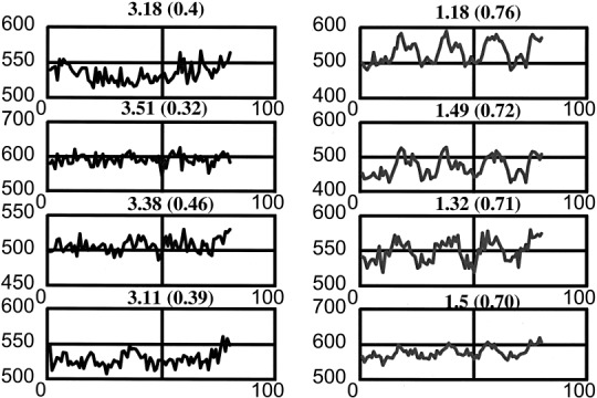
fMRI signals and estimated Renyi entropies for them. The left inset shows the fMRI traces classified as noise by classical correlation coefficient analysis (CC values from top to bottom are 0.04, 0.32, 0.46 and 0.39 respectively). On the right, signals classified as reflecting activation (CC are 0.76, 0.72, 0.76, 0.72), are shown.
For this data set, the Renyi entropy values showed a clear gap between activation and no activation independently of the amplitude of the responses. The appealing aspects in this analysis which contrast with the comparison with a preselected reference vector are twofold: 1) There is no need to guess or model such a reference vector since the classification is based on the counting of the number of elementary components and 2) The method can be applied to experiments where sequences of on‐off conditions are not available.
Still, in the whole analysis of a fMRI (not discussed here) statistical methods will probably be needed to set the threshold between signals and noise (as done in correlation analysis) if a clear gap as the one observed in this example does not appear.
Analyzing Intracranial ERPs
Intracranial ERPs were obtained from 94–100 recording sites of two epileptic patients (A.M. and N.B.). The patients had subdural grids or strips implanted on their left hemispheres as part of presurgical diagnostic investigations including electrical cortical stimulation to map brain functions. After informed consent had been obtained, both patients participated in a study on visuomotor integration. As a part of this study patients performed simple unimanual index finger responses to black dots, which were presented every 5–6 sec for 60 msec in random order either to the left or to the right of a central fixation cross on a gray computer screen. Here two conditions were further evaluated: 1) Right visual field stimulation, right hand response (RR) 2) Left visual field stimulation, right hand response (LR). After having performed a training session, NB was tested in 80 trials per condition and AM in 60.
The EEG was recorded continuously with a sampling rate of 190 Hz (AM) or 200 Hz (NB) in a bipolar montage, bandpass 0.1–100 Hz. EEG was analyzed off‐line and EEG epochs (100 ms before and 500 ms after stimulus onset) were computed and averaged after artifact rejection. Averages were later bandpass filtered (Butterworth) between 1 and 50 Hz. The motor responses recorded with a response key device were situated within the time window of analysis. Mean reaction times were 352.4 ± 76 ms for NB and 257 ± 47 ms for AM.
For each averaged signal, we computed first the scalogram and then the Renyi entropy of order three [Auger et al., 1996]. Figure 5 shows the plot of the values of the Renyi's number superimposed over the grid or stripes in the individual MRIs of the two patients. The darker the region the lower the RE. The regions with the lowest REs were encircled to outline the sites where the most organized responses appeared. For surgical reasons the grid had to be oriented horizontally in NB and vertically in AM. In Figure 4b we display the results of the electrical cortical stimulation. The different symbols represent the brain sites from which visual illusions, right hand somato‐sensory phenomena or right hand movements were elicited. These areas were expected to be activated during the performance of the simple visuomotor reaction time task.
Figure 5.
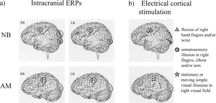
Estimated response complexity in a visuo motor task in two epileptic patients. (a) Calculated Renyi's entropies superimposed on the individual MRIs of the two epileptic patients. The regions with the lowest NNREs (darkest values) are encircled to outline the sites where the most organized and strongest responses appeared. (b) Results of the electrical cortical stimulation. The different symbols represent the brain sites from which visual or right hand somato‐sensory illusions or right hand movements were elicited.
In line with these expectations we found that the regions with highest organized signals in terms of RE correspond for both patients to the contacts over motor and sensory motor areas, and for one patient (NB) to contacts over visual areas. No highly organized signals are observed over the visual areas of AM. However, these contacts lie more anterior than the visual ones in NB, and are thus likely to cover higher order visual cortex not necessarily engaged in visual information processing in this simple task.
Analyzing Time Series Estimated by ELECTRA
While fMRI is able to detect functional activation with excellent spatial resolution, this technique lacks the capability to track neural events at the milliseconds level. Temporal evolution of such events can be traced by electrophysiological techniques such as EEG, ERP or MEG which are nonetheless unable to provide accurate spatial localization. Therefore, there is an increasing tendency to combine both neuroimaging techniques. Such combination generally requires the solution of the electromagnetic inverse problem either using spatio temporal source models or distributed inverse solutions.
One aspect that has somehow limited the combination of fMRI and EEG/MEG inverse solutions is that the relationship between hemodynamic responses and underlying electrophysiological events is not yet clearly established. It is however reasonable to assume that fMRI images provide a coarse temporal average of electrophysiological events. One manner to further assess this hypothesis is to compare for similar experiments fMRI images with temporal averages of intracranial recordings or distributed inverse solutions. While intracranial recordings are usually restricted to a few brain sites in pathological brains, the results of inverse solutions are not always reliable especially in terms of the estimated amplitudes of the deeper sources. Recent simulations have suggested that the temporal courses of the generators tend to be more reliably estimated (except for an amplitude factor) than the instantaneous amplitude map [Grave de Peralta et al., 2000]. This reason speaks in favor of searching for methods to analyze the estimated signals in terms of their temporal organization rather than relying on the instantaneous maps. Obviously the methods to analyze these time series should not depend upon a scale factor which is insured here by the use of equation (3).
We concretely propose to compare fMRI results with the images obtained by determining the traces of the estimated inverse solution which show a consistent activation over time. Activation will be measured trough the Renyi entropy. For simplicity we use a recently developed distributed inverse solution coined ELECTRA [Grave de Peralta and Gonzalez, 1999; Grave de Peralta et al., 2000] which restricts the source model to the kind of currents that can be actually detected by scalp electrodes. Besides it's mathematical properties, ELECTRA is particularly appealing for the analysis described here because it is the first inverse solution that attempts to estimate the three dimensional potential distribution inside the human brain such as the one provided by implanted intracranial electrodes. In this sense ELECTRA's results can be compared with those measured experimentally and all procedures employed to analyze these traces, as the one proposed in this paper, can be applied.
In Figure 6 we present an example of application of the RE to the detection of signals in the potentials estimated by ELECTRA in a simple visual task. In the experimental protocol, 41 channel evoked potentials (EP) were recorded in 25 healthy subjects. Checkerboard reversal stimuli (500 ms) were presented to the left, the center or the right visual field. The mean average response over subjects was computed and ELECTRA solution was obtained for this grand mean data using an spherical volume conductor model of the head.
Figure 6.

The lowest RE values for the time series estimated by ELECTRA in a simple visual task. Top: Right visual field stimulation and Bottom: Central visual field stimulation. Only the four lower slices of the solution space are shown.
Figure 6a and b show the 3‐dimensional RE maps for the right and central visual field stimulation, respectively. The sites with the most organized responses (lower RE) are shown. Consistent with the basic anatomical, electrophysiological and clinical knowledge [Regan, 1989], the lateralized stimuli (right) mainly led to activation of the occipital areas contralateral to the stimulated field, while full‐field stimulation induced symmetrical activation of the occipital areas of both hemispheres.
DISCUSSION
We have described and illustrated here an approach to differentiate activation from noise in neurophysiological signals of diverse origins with minimal assumptions. This approach uses as a measure of activation the RE calculated over the basis of the time frequency representation of the measured signals. Although many additional theoretical properties of the RE are discussed in Baraniuk et al, (submitted), we prefer to discuss here those merits, pitfalls and caveats of more practical relevance. It should not be neglected that the lack of uniqueness in this definition of complexity given its dependence of the selected TFR is an obvious theoretical flaw of this method. More relevant on practical grounds are the presence of cross‐components or interference terms in the TFR which affect the counting property of the RE. Also amplitude and phase differences between the components of the signal alter the asymptotic saturation levels as illustrated in Figure 2. This is why the selection of an adequate TFR, able to extract the relevant features of the signal to be processed with a minimum of interference terms, is a crucial aspect in the analysis proposed. Probably even more important than the selection of the TFR itself is the adequate tuning of its parameters taking into account the unavoidable trade off between time and frequency resolution. On one hand, a good time resolution requires a short temporal analysis window; on the other hand a good frequency resolution requires a long time window. Unfortunately both wishes cannot be simultaneously granted. In the particular case of ERPs and fMRI signals it can be assumed that their frequency changes over time are not very fast and thus the time resolution is not as important as the frequency resolution [McGillem and Aunon, 1987]. Consequently, in this case a long temporal window can be chosen which might not be adequate for other types of data.
It is also relevant that this measure of complexity is closely related to our intuitive notion of organization of the signals. If the TFR adequately separates the elementary components of the signals in the time frequency plane, then this measure reflects more or less adequately the number of components. Usually, the more peaky time frequency representation of signals comprised of small numbers of elementary components yield small entropy values (small Renyi numbers), while the diffuse TFRs of more complicated signals yield large entropy values (large Renyi numbers).
One could also wonder if other measures derived from the TFR of a signal such as moment‐based measures, e.g., time‐bandwidth and its generalizations to second order time frequency moments could replace the RE as measures of complexity. A simple example described by Baraniuk (submitted) shows that this is not the case. Let's consider a signal comprised of two components of compact support, i.e., which are zero outside a certain region of the time frequency plane. While the time‐bandwidth product increases without bound with separation, the complexity does not increase once the components become disjoint as illustrated in the basic theory section.
Alternative measures of complexity have already been applied to the analysis of electrophysiological signals [Wackermann et al., 1993; Tononi et al., 1996; Aftanas et al., 1998; Micheloyannis et al., 1998; Weber et al., 1998 among others]. Most of these measures are derived in the context of non linear analysis and chaos [Cerutti et al., 1996] and are difficult to apply to general neurophysiological signals. The main reason is that an adequate estimate of the complexity requires a large number of samples, i.e., either signals sampled at a very high sampling frequency or very long periods. These conditions are not always fulfilled in practice. Additional difficulties of using non linear analysis techniques are described in Nunes [1995].
The applications described and illustrated here merely scratch the surface of potential applications of TFRs or RE for the analysis of brain signals. An interesting potential application is to exploit the “analogy” TFR and probability density for the calculation of the average amount of mutual information, a measure of the interdependence between time series applicable to the study of information transmission between brain areas [Mars and Da Silva, 1987]. A generalization of the Shannon measure known as the Gelfand and Yaglom measure have been already used in the EEG/ERP literature to study the structure of brain interdependencies [Mars and Da Silva, 1987, for a review]. An understanding of the principles governing the behavior of epileptiform activity, where the complexity is reported to decrease preceding the seizure [Lehnertz et al., 1997; Weber et al., 1998] or the analysis of changes and transitions of the brain electric activity before and after drugs intake can be obtained from the application of the methods described here.
CONCLUSIONS
In this paper we describe a measure of the complexity of neurophysiological signals: the Renyi entropy. This measure is conceptually simple to understand and as illustrated in the analysis of several types of neurophysiological signals, it corresponds well with our visual notion of complexity. In contrast with measures derived in the framework of non linear analysis this measure does not require long time series. Worthy to note is that this method implies nearly no assumptions about the underlying processes or the recorded signals, which makes this measure of complexity robust and generally applicable. All these properties are essential for the analysis of the diverse signals arising from different modalities of brain imaging which describe very different neurophysiological processes.
Our goal with this paper is not to describe an approach able to access information invisible to other methods. We aim instead to describe a tool to extract the same information with less assumptions. It is important to realize that most of the standard methods available to distinguish signals from noise imply requirements such as gaussianity or stationarity, demand lengthy time series or presuppose some a priori knowledge about the underlying neurophysiological process. Many of these hypothesis do not necessarily hold for each neuroimaging modality or for each experimental paradigm, and their validity is hardly ever tested in practice. Therefore, a method like the one proposed here, general enough to handle a multiplicity of neurophysiological signals without needing assumptions about them, should not be disregarded.
Acknowledgements
Work supported by the Swiss National Foundation Grants 4038‐044081, and 21‐45699.95
REFERENCES
- Aftanas LI, Lotova NV, Koshkarov VI, Makhnev VP, Mordvintsev YN, Popov SA (1998): Non‐linear dynamic complexity of the human EEG during evoked emotions. Int J Psychophysiol 28(1): 63–76. [DOI] [PubMed] [Google Scholar]
- Auger F, Flandrin A, Goncalves P, Lemoine O (1996): Time Frequency Toolbox for use with Matlab.
- Baker J, Weisskoff R, Stem C, Kennedy D, Jiang A, Kwong K, Kolodny L, Davis T, Boxerman J, Buchwinder B, Wedeen B, Bellivau J, Rosen B (1994): Statistical assessment of functional MRI signal change. In: Proceedings of the second annual meeting of the society of magnetic resonance, p 626.
- Bandettini PA, Jesmanowicz A, Wong EC, Hyde JS (1993): Processing strategies for time‐course data sets in functional MRI of the human brain. Magn Res Med 30: 161–173. [DOI] [PubMed] [Google Scholar]
- Baraniuk RG, Flandrin P, Hansen AJEM, Michel O (submitted): Measuring time frequency information content using the Renyi entropies. Postscript version available at http://www-dsp. rice.edu/publications.
- Bodreaux‐Bartel GF (1996): Mixed time‐frequency signal transformations In: The transforms and applications handbook ( Poularikas, Ed.) pp. 887–963. Boca Raton‐CRC Press. [Google Scholar]
- Cerutti S, Carrault G, Cluitmans OJ, Kinie A, Lipping T, Nikolaidis N, Pitas I, Signorini MG (1996): Non‐linear algorithms for processing biological signals. Comput Methods Programs Biomed 51: 51–73. [DOI] [PubMed] [Google Scholar]
- Flandrin P, Baraniuk RG, Michel O (1994): Time frequency complexity and information. Proc IEEE Int Conf Acoust, Speech, Signal Processing‐ICASSP'94. III: 329–332.
- Grave de Peralta Menendez R, Gonzalez Andino SL (1999): Distributed source models: Standard solutions and new developments In: Uhl C, ed. Analysis of Neurophysiological Brain Functioning. Heidelberg: Springer Verlag. [Google Scholar]
- Grave de Peralta Menendez R, Gonzalez Andino SL, Morand S, Michel CM, Landis TM (2000): Imaging the electrical activity of the brain: ELECTRA. Hum Brain Mapp 9(1) 1–12. [DOI] [PMC free article] [PubMed] [Google Scholar]
- Gersch W (1987): Non‐stationary multichannel time series analysis In: Handbook of Electroencephalography and Clinical Neurophysiology. ( Gevins AS, Remond A, eds) Vol. 1, Methods of Analysis of Brain Electrical and Magnetic Signals Amsterdam‐New York‐Oxford: Elsevier; p 261–296. [Google Scholar]
- Lange N, Zeger SL (1997): Non linear Fourier time series analysis for human brain mapping by functional magnetic resonance imaging. Journal of the Royal Statistical Society. Series C, Applied Statistics, 46(1) p 1–30. [Google Scholar]
- Lehnertz K, Elger CE, Weber B, Wieser HG (1997): Neuronal complexity loss in temporal lobe epilepsy: effects of carbamazepine on the dynamics of the epileptogenic focus. Electroencephalogr Clin Neurophysiol 103(3): 376–380. [DOI] [PubMed] [Google Scholar]
- Lin Z, Chen JD (1996): Advances in time‐frequency analysis of biomedical signals. Crit Rev Biomed Eng 24(1): 1–72. [DOI] [PubMed] [Google Scholar]
- Mars NJ, Lopes da Silva FH (1987): EEG analysis methods based on information theory In: Handbook of Electroencephalography and Clinical Neurophysiology. ( Gevins AS, Remond A, eds) Vol. 1, Methods of analysis of Brain Electrical and Magnetic Signals Amsterdam‐New York‐Oxford: Elsevier; p 297–307. [Google Scholar]
- McGillem CD, Aunon JI (1987): Analysis of event‐related potentials In: Handbook of Electroencephalography and Clinical Neurophysiology. ( Gevins AS, Remond A, eds) Vol. 1, Methods of analysis of Brain Electrical and Magnetic Signals Amsterdam‐New York‐Oxford: Elsevier; p 131–170. [Google Scholar]
- Micheloyannis S, Flitzanis N, Papanikolau E, Bourkas M, Terzakis D, Arvanitis S, Stam CJ (1998): Usefulness of non‐linear EEG analysis. Acta Neurol Scand. 97 (1): 13–9. [DOI] [PubMed] [Google Scholar]
- Nunes PL (1995): Non linear analysis and chaos In: Neocortical dynamics and human EEG rhytms. (Nunes PL, ed). New York‐Oxford: Oxford University Press; p 417–474. [Google Scholar]
- Regan D (1989): Human Brain Electrophysiology. Elsevier. [Google Scholar]
- Renyi A (1961): On measures of entropy and information. In: Proc. 4th Berkeley Symp. Math. Stat. and Prob. Vol. 1, p 547–561.
- Ruttimann UE, Unser M, Rawlings RR, Rio D, Ramsey CNF, Mattay VS, Hommer DW (1998): Statistical analysis of functional MRI data in the wavelet domain. IEEE Trans. Medical Imaging, 17(9) p 2555–2558. [DOI] [PubMed] [Google Scholar]
- Shannon CE (1948): A mathematical theory of communication. Part I, Bell Sys Tech J 27: 379–423. [Google Scholar]
- Tononi G, Sporns O, Edelman GM (1996): A complexity measure for selective matching of signals by the brain. Proc Natl Acad Sci USA. 93(8): 3422–7. [DOI] [PMC free article] [PubMed] [Google Scholar]
- Unser M, Aldroubi A (1996): A review of wavelets in biomedical applications. Proc IEEE, vol. 84, p 626–638. [Google Scholar]
- Wackermann J, Lehmann D, Michel CM (1993): Global dimensional complexity of multichannel EEG indicates change of human brain functional state after single dose of a nootropic drug. Electroenceph Clin Neurophysiol 86: 193198. [DOI] [PubMed] [Google Scholar]
- Weber B, Lehnertz K, Elger CE, Wieser HG (1998): Neuronal complexity loss in interictal EEG recorded with foramen ovale electrodes predicts side of primary epileptogenic area in temporal lobe epilepsy: a replication study. Epilepsy, 39(9): 922–7. [DOI] [PubMed] [Google Scholar]
- Willians WJ, Brown ML, Hero AO (1991): Uncertainty, information and time‐frequency distributions. In: Proc SPIE Int Soc Opt Eng, vol. , p 144–156. [Google Scholar]
- Worsley K, Friston K (1995): Analysis of fMRI time series revisited‐again. Neuroimage 2: 173–181. [DOI] [PubMed] [Google Scholar]
- Xiong J, Gao JH, Lancaster JL, Fox PT (1996): Assessment and optimization of fMRI analysis. Hum Brain Mapp 4: 153–167. [DOI] [PubMed] [Google Scholar]