

Abstract
A methodology for fMRI data analysis confined to the cortex, Cortical Surface Mapping (CSM), is presented. CSM retains the flexibility of the General Linear Model based estimation, but the procedures involved are adapted to operate on the cortical surface, while avoiding to resort to explicit flattening. The methodology is tested by means of simulations and application to a real fMRI protocol. The results are compared with those obtained with a standard, volume‐oriented approach (SPM), and it is shown that CSM leads to local differences in sensitivity, with generally higher sensitivity for CSM in two of the three subjects studied. The discussion provided is focused on the benefits of the introduction of anatomical information in fMRI data analysis, and the relevance of CSM as a step toward this goal. Hum. Brain Mapping 12:79–93, 2001. © 2001 Wiley‐Liss, Inc.
Keywords: statistical analysis, cortical surface, spatial smoothing, fMRI, methodology
INTRODUCTION
Data analysis of functional magnetic resonance imaging (fMRI) protocols is currently done with little regard for the anatomical specificity of the object under study. Even though simple operations based upon anatomical information are occasionally performed (e.g., threshold‐based masking out of extracerebral voxels), usually no attempt is made to take into consideration the spatial distribution of the different tissues (grey and white matter) involved, nor particular topological specificities such as the sheet‐like near‐2D nature of the cortex. In most implemented procedures, signal emanating from grey and white matter is treated in an indiscriminating fashion, and the spatial smoothing step very often included in the analysis chain leads to nuisance averaging with surrounding, non‐interest signal, and most particularly with extracerebral signal, potentially harming analysis sensitivity. Moreover, the highly convoluted structure of the cortex will inevitably lead to situations of smoothing‐induced signal averaging across sulci, reducing spatial discriminating power. Making the entire data analysis chain of procedures more compliant with the structure of the cortex thus appears as a natural and highly desirable step.
Anatomical representations of the cortex, obtained from segmented T1‐weighted magnetic resonance images (MRI), have sometimes been used as an aid to fMRI data analysis. Retinotopy studies in humans, for instance, have resorted to cortical representations to assist the mapping of visual cortex topographic organisation [Sereno et al., 1995; DeYoe et al., 1996], and smoothing over the cortical surface has been proposed to help with the visualisation of the spatial organisation of the visual areas [Tootell et al., 1997]. Indeed, the definition of surface‐based coordinate systems provides a more natural framework for cortically oriented analyses. Recently, surface‐based coordinate systems have been further used to facilitate the building of probabilistic atlases for large populations [Fischl et al., 1999]. These efforts have often been associated with the development of flattening or unfolding techniques [Drury et al., 1996; Fischl et al., 1999].
However, it remains that representations of the cortex have mostly been used as a tool to help gain a richer and more encompassing perspective over results obtained in the classical, 3D‐based fashion. Techniques for performing detection over the cortex have been devised [Goebel and Singer, 1999], but so far lack generality and have not yet gained widespread acceptance. Recently, a new approach aiming to introduce a certain amount of 2D cortical anatomy information in functional brain data analysis, through the use of anatomically constrained spatial basis functions has been presented [Kiebel et al., 2000]; see also [Poline et al., 1995]. It is conceptually close to deconvolution techniques, and it has the merit of providing a strictly two‐dimensional framework, thereby shifting the focus from 3D space to cortical space. Nevertheless, an integrated methodology to perform strictly two‐dimensional fMRI data analysis, able to tackle problems such as surface spatial smoothing and multiple comparisons correction, while avoiding the problems stemming from the metric distortion that is a result of explicit flattening techniques, had yet to be developed.
In the present paper, we propose a methodology (Cortical Surface Mapping, or CSM for short) meant to allow for a more extensive introduction of anatomical information throughout the analysis of fMRI experiments. In its essence, CSM closely follows standard approaches that rely upon General Linear Model parameter estimation, voxel‐by‐voxel hypothesis tests, and the building of statistical parametric maps [Friston et al., 1995; Worsley et al., 1992], as it is implemented, for instance, in the SPM package, but several adaptations are introduced to take into account the near‐2D nature of the cortex as well as its convoluted structure. In this work, the proposed CSM methodology is tested on simulated noise data and its sensitivity is studied with a motor protocol (grasping). The results are compared to those obtained with standard 3D SPM on the same data.
MATERIALS AND METHODS
Description of the Proposed Methodology
General Overview
CSM methodology can be subdivided into several stages. The procedures involved, which are briefly described below, are either common to standard, 3D‐oriented methods or require adaptations, to a greater or lesser extent. Important conceptual differences with respect to standard methods are presented in a separate treatment of the procedures in question. The stages comprise:
Spatial image transformation(s): The set of functional MRI scans acquired in the course of the experimental protocol can be spatially realigned and/or normalised to match a template. These are optional spatial transformations, and the decision to apply one or both should be guided by criteria (subject motion, purpose of making inter‐subject comparisons) that have no direct bearing upon the specific nature of the proposed methodology. Coregistration between the T‐weighted scans and a T1‐weighted anatomical scan can be performed to ensure a satisfactory match between the cortical representation (obtained from the T1‐weighted image) and the functional volumes. The assignment of values to cortical positions (see below) relies heavily upon this matching; therefore this is a critical step. However, coregistring is not compulsory, provided that no substantial subject movement takes place between the functional and anatomical acquisitions. Distortion in the functional scans, due to Echo‐Planar acquisition, is also a major issue, since it can put in jeopardy the possibility of achieving a satisfactory match. For moderate field MRI machines, distortion should not be strong enough to require the application of a correction algorithm [Jezzard and Clare, 1999].
Grey matter/white matter segmentation: Grey and white matter masks are built through segmentation of the T1‐weighted anatomical scan of the subject [Mangin et al., 1995].
Surface extraction: A triangulated lattice representation of the internal surface of the cortex is extracted, through application of a surface tracking algorithm to the white matter segmented volume [Gordon and Udupa, 1989]. The lattice comes under the form of a very dense mesh (the node separation is of the order of the anatomical acquisition voxel size, typically ∼1 mm), with a size that varies typically between 100,000 and 150,000 nodes for each hemisphere. Constraints in the segmentation method insure that the lattice is homotopic to a sphere.
Value assignment to the surface positions: The T‐weighted functional scans are interpolated on the positions corresponding to the nodes of the cortical lattice (plus a user defined outward shift in the surface normal direction to account for cortical thickness). The outcome of this operation is a set of cortical surface scans (CS‐scans) with n values, n standing for the number of nodes in the cortical lattice. Each value is associated with a set of coordinates corresponding to the interpolating position. Subsequent analysis steps will thus be confined to a set of values interpolated from the neighbourhood of the cortex.
Spatial smoothing: Each one of the CS‐scans, consisting of a set of values associated with node positions, is spatially smoothed. While the purpose behind this surface‐based smoothing is essentially the same as for the classical 3D analysis, the conceptual basis of its implementation is markedly different, and therefore this step is treated in more detail below.
General Linear Model parameter estimation: Estimation is performed in essentially the same way as with classical three‐dimensional analysis. The option to perform global correction (proportional scaling) or temporal filtering is retained. The output is a set of estimated parameters, with the same dimension (i.e., number of nodes) as an individual functional CS‐scan.
Smoothness estimation: For this step, we have employed “statistical flattening” [Worsley et al., 1999], a generalised estimation procedure that takes into account local fluctuations of smoothness, and is easily adaptable to the particular requirements of the proposed methodology. This procedure and its implementation receive a more thorough (albeit informal) independent treatment below.
Hypothesis testing based on intensity: The assignment, for each node, of a P value reflecting the risk of error concerning the rejection of a null hypothesis involving a linear combination of the estimated parameters is based upon the theory of random fields, and does not differ from currently employed procedures [Friston et al., 1995; Worsley et al., 1996b].
Surface‐based Smoothing
The purpose behind spatial smoothing of functional brain imaging data is two‐fold [Petersson et al., 1999]:
Improving signal‐to‐noise ratio, through the use of a smoothing kernel wide enough to filter out a significant part of the (mostly high‐frequency) noise.
Ensuring that the output field of values constitutes an adequate discrete representation of a continuous statistical field, so that subsequent inference procedures based on the theory of random fields are valid. For this to be achieved, the smoothness of the field must be large compared to the sampling resolution of the images under study. Note that this is not an absolute constraint, since subsampling can always be employed as a way to impose the required conditions.
Smoothing is usually implemented as a simple, fully isotropic convolution with a three‐dimensional Gaussian kernel, and it is applied uniformly over the entire volume. Such an implementation does not take into account the anatomical configuration of the brain (different kinds of tissue, deeply folded structure, etc.). This leads to averaging of signal emanating from the cortex and from while matter of CSF, as well as to averaging of signal issuing from sources that are close to each other in a Euclidean sense, but geodesically far apart. CSM methodology implements surface‐oriented smoothing, aiming to obtain a spatial correlation structure that depends on geodesic rather than Euclidean distance. In this way, the introduction of artificial correlation between areas that are close together in Euclidean terms but geodesically far apart (e.g., two points on opposite sides of a sulcus) is avoided.
This implementation of surface‐oriented smoothing differs from simple, voxel‐based isotropic three‐dimensional convolution in two main aspects:
At the practical level: smoothing is applied to a field of values sampled with an irregular grid (as opposed to a regular voxel‐based sampling).
At the conceptual level: smoothing is done along the cortical surface, instead of being extended to the whole acquired volume.
Clearly, convolution with a Gaussian kernel is no longer a viable choice: the highly convoluted nature of the cortex, along with the irregular sampling, requires a new theoretical framework to build the smoothing procedure upon.
Smoothing an irregularly sampled field of values
The solution adopted to take the irregularity of the sampling grid into account relies on a result widely employed in image processing [Koenderink, 1984]: the equivalence between Gaussian convolution and heat diffusion. The diffusion of heat in a time‐varying field of temperatures I(r→, t) proceeds according to a law expressed as
| (1) |
where t is time, K is a constant involving several physical parameters (K = c/ρcp, with c standing for thermal conductivity, ρ for density and c p for specific heat), and ∇2 is the Laplacian operator (∇2 I(x, y) = ∂2I/∂x2 + ∂2I/∂y2, in two dimensions). This assumes that K is constant all over the field. On the other hand, if t is taken to represent a smoothness (scale‐space) parameter, instead of time, it can be proved that
(convolution of an image I(r→,t = 0) with a Gaussian kernel) is a solution of Equation 1 (with K = 0.5). Hence, applying a Gaussian spatial filter with parameter  to an image is the same thing as letting a diffusion process run its course for a lapse of time T. The advantage of this formulation based on a differential equation is that it lends itself more easily to being adapted for the specific case of an irregular 2D lattice embedded in a three‐dimensional space.
Numerical computation of the results of a diffusion process over a discrete field of values can be carried out as an iterative process of the form
| (2) |
for each temporal iteration step (Δt).  is the local estimation of the Laplacian at time t. The application of this solution would be trivial in the case of a regular lattice with a fixed neighbourhood: finite differences, for instance, could be chosen as a method for locally estimating partial derivatives. For an irregular lattice, a general approach can be employed [Liszka and Orkisz, 1980; Huiskamp, 1991], based on the Taylor series expansion of a function around a point. Assume that an image, implicitly described by a function I(x, y), is sampled with an irregular lattice composed of interconnected nodes. For a point (x0,y0) of the image, this expansion has the form:
 |
(3) |
where Ii = I(xi, yi), hi = xi − x0, ki = yi − y0, and  . Writing Equation 3 for a surface element consisting of a lattice node, located at (x
0, y
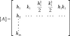
0), and its neighbours i = 1, 2,…m, we obtain the set of equations
. Writing Equation 3 for a surface element consisting of a lattice node, located at (x
0, y
0), and its neighbours i = 1, 2,…m, we obtain the set of equations
where
 |
and the five derivatives at point (x0, y0) are
In this fashion, estimates of the two‐dimensional Laplacian (∇2 I(x, y) = ∂2 I/∂x2 + ∂2 I/∂y2) are obtained at each node of the lattice. This approach amounts to solving, for each node, a linear system involving the relative positions of the node and its neighbours and the corresponding field value differences. It is still a finite differences method, in the sense that the partial derivatives are estimated by differences between field values in neighbouring points, but its range of application is extended to any arbitrarily irregular grid. Some constraints remain, however, concerning the configuration of the lattice. Firstly, the application of post‐processing procedures (e.g., decimation) to the lattice may lead to situations in which node neighbours are fewer than the number of variables estimated locally (this number will be 5 in the case of the second order Taylor expansion necessary to estimate the Laplacian, or 4 if isotropy is assumed and the ∂2f0/∂x∂y term is considered to be zero), making the corresponding linear system underdetermined, which means that the solution will not be unique. One of the options to pick one among the infinity of solutions thus obtained is to select the solution with the smallest norm. This is the condition implied by the pseudo‐inverse based resolution that we adopted. This was shown to be a sensible option in practice: provided that the nodes with less than four neighbors constitute a small (∼1%) proportion of the total number of nodes, the final results do not differ significantly from those obtained in a situation of system determinacy all over the lattice. The second constraint has to do with node separation: the nodes must be sufficiently close together for the partial derivative estimations to be reliable. The specifics of lattice building are not discussed in this paper, but it should be made clear that these constraints can be applied at the surface extraction stage, by suitable tuning of the extraction algorithm parameters. In the analyses we carried out, we employed both undecimated lattices (the direct output of the surface extraction stage), with ∼100,000–150,000 nodes per hemisphere, and lattices that underwent constrained node decimation. The latter had ∼25,000 nodes per hemisphere, and a small (<1%) proportion of nodes with less than four neighbours. Mean and maximal internodal distance were, respectively, 1 and 1.8 mm (undecimated lattice) and 2.5 and 6 mm (decimated lattice). Only minor differences were detected between the results obtained with undecimated and decimated lattices. This seems to indicate that the presence of important internodal distance variability, and the resulting local decrease in the accuracy of Laplacian estimation, does not per se affect the outcome of the analysis in a significant way.
Another important concern is the choice of the temporal iteration step (Δt in Equation 2). The critical value above which the numerical resolution will be unstable [Press et al., 1992; Gerig et al., 1992], in the specific case of the diffusion equation, depends on thermal conductivity, a parameter included in the K term in Equation 1. In the case of diffusion‐based smoothing over a lattice, this conductivity term can be seen as conceptually equivalent to node distance: the closer a pair of nodes is, the stronger their mutual influence, and this mimics the situation of high thermal conductivity and fast heat propagation. Irregular node spacing, thus, parallels a situation of varying thermal conductivity across the field. The critical temporal iteration step is directly proportional to the minimal node distance, because instability tends to spread over the whole lattice, and therefore a single pair of nodes that are too close together will be enough to globally affect the results. Lattices possessing nodes in these conditions require very small temporal iteration steps, and this may lead to exceedingly long processing times. Hence, a double constraint operates at the level of node separation: small internodal distances imply a small temporal iteration step and long computation times; on the other hand, very large internodal distances will eventually affect the reliability of the Laplacian estimations. There is, thus, a trade‐off between processing speed and estimation accuracy.
If computation time is not unreasonably large, a conservative value for Δt should be chosen. We have adopted a default value of Δt = 0.1, throughout the analysis of the fMRI protocol described below, which proved to be low enough to lead to a stable process for the undecimated lattices we worked with (minimal internodal distance ∼0.6–0.7 mm). For these very dense lattices (∼100,000–150,000 nodes), this choice implies that a diffusion process equivalent to convolving with a Gaussian kernel with FWHM = 8 mm (σ = 3.397) requires 115 iterations (that is σ2/Δt rounded to the nearest integer). In terms of computation time, this represents roughly 2–3 min in a SUN ULTRA 10 workstation, for a single CS‐scan (one hemisphere). Grouping scans in blocks treated simultaneously allows to optimise smoothing time, so that the increase in time is not linear with respect to the total number of scans. 8 mm smoothing for a protocol consisting of ∼100 scans takes a few hours, making this by far the most time‐consuming step of the analysis. Computation time may quickly rise to prohibitive values for bulkier protocols, and this is why the use of decimated lattices may be recommended, or even become compulsory. To give an idea of the decrease in computation time, the same amount of smoothing applied to the same protocol, but this time with scans built from decimated lattices (∼25,000 nodes) took ∼40 min.
Smoothing Along a Curved Surface
The theoretical framework described in the previous paragraph was chosen to tackle the problem of smoothing an irregularly sampled field of values. We have focused on its 2D version, since the aim is to smooth over the surface. However, the fact that the cortical representation lattice is embedded in a volume raises a problem concerning the proper axis system upon which to base the estimation of the local partial derivatives. A conflict exists between the need to employ three spatial coordinates in the Euclidean space to unambiguously describe the position of each node and the wish to perform a strictly surface‐based smoothing: locally estimating three‐dimensional Laplacians and solving the diffusion equation accordingly would clearly go against this intent. The definition of a coordinate system intrinsic to the surface would allow for a strictly 2D‐based smoothing. This implies a parameterization, i.e., the definition of a mapping function m such that (x, y, z) ≡ m−1 (u, v), u and v being the new coordinates that allow to refer to every point in the surface without ambiguity. The diffusion equation is then solved along u and v, in a strictly 2D fashion.
The parameterization adopted was a simple local transformation that maps each surface element (a node and its first neighbours) into the plane, while keeping unchanged both the edge distances and the angular proportions between the edges [Welch and Witkin, 1994]. An individual mapping function m i is defined for each node i, independently of the surrounding surface elements. This approach is made possible since, for each iteration step of the numerical solution of the diffusion equation, the estimations involve only the differences between the values associated with each node and its nearest neighbours. Locally mapping each surface element into the plane avoids the severe areal distortion that would result from a global flattening. This distortion is of the order of 10–20% [Drury et al., 1996], but locally attains much higher values.
Multiple Comparisons Correction by Means of “Statistical Flattening”
Statistical inference of parametric maps must take into account the degree of effective mutual dependence presented by the individual hypothesis tests. Considering the tests as totally independent would not be realistic, since, due both to physiological reasons and to instrumentation‐related specifics of fMRI acquisition, a certain amount of correlation will always be present, and hence a Bonferroni‐type correction would generally prove too harsh [Worsley et al., 1992]. Usually, an estimation of the field smoothness is made, and the stringency of the correction depends upon this measure of spatial correlation.
Smoothness‐based correction can be seen as the computation of the number of tests normalised for the global smoothness of the statistical field. This can alternatively be seen as “shrinking” the field so that its extent, in each of the space directions, is expressed in smoothness‐normalised Resolution Elements (Resels) [Worsley et al., 1992] instead of voxels. An intuitive generalisation of this principle consists in the estimation of local smoothness parameters, and in locally shrinking the field so that distances are normalised for the smoothness estimation at that point. This, in very general terms, is the idea behind the “statistical flattening” correction procedure, described elsewhere [Worsley et al., 1999], and chosen to implement multiple comparisons correction in the cortical surface mapping methodology described herein. This procedure applies local smoothness estimations based on the residual values, after removal of the effects accounted for by the experimental linear model. To permit exact flattening, this operation takes place in the multidimensional residual space, impossible to visualize, into which the individual values are mapped.
Although statistical flattening can be applied in the case of standard volumic analyses (it has, indeed, been incorporated to the latest release of the SPM package), it lends itself particularly well to being adapted for the case of data associated with a triangulated lattice: edge distances are normalised by the correlation between the normalised residuals associated with the corresponding nodes, so that the ensuing correlation structure is isotropic, and the total surface of the deformed field reflects the number of effectively independent tests involved.
Validation with Simulated Noise Scans
To assess the type I error of the implemented method, CSM analysis methodology was validated using random noise scans and a simulated protocol. Twenty random noise volumes (mean μ = 0) were interpolated on an irregular lattice (586 nodes), and the resulting sets of values underwent the treatment described above. Two different values of surface‐based smoothing were applied, corresponding to equivalent Gaussian kernels with an FWHM of 5 and 8 mm. A total of 500 noise sets were generated and analysed, and the ensuing t statistics were converted to corrected intensity‐level P values. Since exact results for the P value of the maximum of a statistical field are not known, P value computation resorted to the expected Euler characteristic of a thresholded field [Worsley et al., 1996b]. Multiple comparisons correction was performed using the previously described procedure (“statistical flattening”).
For each of a set of thresholds ranging from α = 0.01 to α = 0.20, the number of suprathreshold regions due to noise was computed for each of the 500 simulated analyses, for each amount of smoothing, to check how closely the observed number of spurious activations followed the theoretical false positive rate.
Application to an fMRI Protocol
Surface‐based analysis was applied to data from three subjects that took part in a motor (grasping) activation experimental protocol, consisting of three activation epochs separated by three rest periods. Acquisitions were made on a GE 1.5 T machine, using an Echo‐Planar Imaging sequence (TR = 2 s, image matrix 64 × 64 × 18, functional voxel size 3.75 × 3.75 × 3.8 mm3). It was judged that distortion at this moderate field intensity was not important enough to require the application of a correction procedure.
The whole procedure outlined in the General Overview was applied to the three subjects. Realignment was performed only when motion was greater than 1 mm (translation) or 0.5° (rotation) (one subject out of the three). No anatomical normalisation was performed. The matching between the functional volumes and the T1‐weighted, high‐resolution anatomical scan acquired on the same occasion was checked visually.
The cortical triangulated representations (grey matter/white matter interface) were extracted from segmented white matter images obtained from T1‐weighted anatomical scans acquired for each subject. The surface extraction procedures were applied separately for each hemisphere. The results herein presented concern an analysis with undecimated lattices (that is the direct output of the extraction procedure, with no further post‐processing), even though it was verified that the use of decimated lattices was perfectly feasible and gave rise to virtually identical results. The analysis was carried out in parallel for the two hemispheres, and merging occurred only at the statistical analysis stage. This considerably alleviates the computational load, and poses no particular processing or conceptual problem, inasmuch as the hemispheres can be considered to be strictly independent regions, topologically homotopic to a sphere. Smoothing in particular, since it is confined to the cortical surface, should not “spill over” to the opposite hemisphere.
The nodes of the triangulated surface were shifted outward by a distance of 1.5 mm in the normal direction, prior to the interpolation of the functional scans. This represents half an assumed average cortical thickness of 3 mm. Through visual inspection, it was verified that interpolation positions fell inside the functional volume. Figure 1 depicts node positions (after the shift), for a hemisphere, for subject 1, superimposed over a functional scan. This allows for an overall perspective of the matching between the interpolating lattice and the T‐weighted scan. The matching is further illustrated by means of an overlay of the shifted lattice over the anatomical scan (Fig. 2). Note that apparent discontinuities in the lattice surface outline in Figures 1 and 2 do not result from inadequate coverage of the cortical surface by the lattice nodes. They are a consequence of the nearest‐neighbour interpolation step involved in building the volume representation of the lattice. Since internodal spacing is of the order of the anatomical voxel size, the number of voxels that do not contain any node will be considerable, and these appear as gaps in the displayed lattice contour.
Figure 1.

Match between interpolating lattice (originally extracted from anatomical image) and functional scan (for subject 1). Lattice nodes (after shift in normal direction to account for cortical thickness) are shown in a lighter shade, superimposed over coronal, sagittal, and transverse views of a T‐weighted functional scan. Note that apparent discontinuities in the lattice surface outline are due to the interpolation step (see text for explanation).
Figure 2.

Left: Lattice nodes overlayed on sections of anatomical scan (for subject 1). Right: Detail of axial section. Note that apparent discontinuities in the lattice surface outline are due to the interpolation step (see text for explanation).
A simple trilinear interpolation was performed to assign values to the lattice nodes. In the spatial smoothing stage, the lapse of time t for the diffusion process (see Eq. 1) was made to correspond to an equivalent Gaussian kernel with a FWHM of 8 mm. The experimental model comprised the rest and grasping periods (as a boxcar convolved with an estimation of the hemodynamic response function), along with the mean and temporal derivatives.
In parallel, SPM analysis of the same data was carried out with a similar model. The analysis parameters were the same, and the FWHM of the Gaussian kernel used for smoothing was also 8 mm.
Visualisation of the Results
Visualisation of the results resorts to inflated representations of the cortex, to allow for the display of the entire surface, and to provide a clearer picture of sulcal topography. The cortical representations are the same ones that were used for the analysis itself. The adopted implementation for inflation of the cortical triangulated lattices is based on criteria described in the literature [Van Essen et al., 1998; Carman et al., 1995]. The main concern is to minimise metric distortion, while making sure that the whole of the buried cortical structures is brought to light. Since this inflation procedure was devised only for displaying purposes, however, minimisation of metric distortion is not as crucial as in the case of surface‐based analytical procedures (e.g., smoothing, as described above).
RESULTS AND DISCUSSION
Simulations
As illustrated in Figure 3, the false positive rates (spurious activations due to noise) do not stray significantly from the theoretically expected values, for the range of thresholds tested (this range was chosen to span the range of thresholds usually applied in real experiments). This establishes that the statistical flattening procedure, applied to the specific case of a 2D triangulated lattice, is a sound solution to implement multiple comparisons correction, and indicates that protection against type I error is satisfactory, for this intensity‐based test.
Figure 3.

Expected (dashed line) vs. observed (solid line) false positive rate for simulations. 5 mm (top) and 8 mm (bottom) surface‐based equivalent smoothing kernels. Corrected thresholds range from 0.01 to 0.2.
fMRI Protocol
To summarise the results obtained, the following information is presented:
display of activated regions superimposed over inflated representations of the cortex
comparative tables of results obtained with CSM and classical 3D‐based SPM, for one of the subjects
graphics summarising overall reproducibility information, for all three subjects.
The display of activated regions, for both SPM and CSM, over inflated representations of the cortex (Fig. 4) provides an immediate visual check of overall reproducibility. (Only the left cortex is shown.)
Figure 4.

Activated (P < 0.05 corrected) regions superimposed over inflated representations of the left cortex, for the three subjects (top to bottom). Left column: CSM results. Right column: SPM results. The background is a map of curvature signs, making it possible to distinguish the contours of sulci (negative curvature, darker shade) and gyri (positive curvature, lighter shade). Blobs are semi‐transparent to avoid completely blotting out sulcal limits. The colour scale shown for each subject is the same for both modalities (CSM and SPM).
The cortical representations that are shown inflated in Figure 4 are the same ones that were used, before inflation, in the CSM analysis itself. Visualisation of the CSM results relies on a simple one‐to‐one assignment of the t values to the corresponding lattice nodes. For the results of the SPM analysis, the activated voxels corresponding to the chosen threshold were saved as an image, which was subsequently interpolated (trilinear) with the cortical representation used for display, so that t values could be assigned to its nodes. The use of a different interpolation strategy would clearly cause localised changes in the images. For the purposes of qualitative comparison of general activation patterns, however, this should not be a crucial point.
From Figure 4 it is seen that no major disparities exist between the overall activation patterns obtained with SPM and CSM. An extensive parietal activation, as well as sparser frontal ones, are clearly visible in the results of both methods. Results for the right hemisphere (not shown) confirm this observation. As a further corroboration, the averages of the obtained t values were almost similar for both analyses: for instance, the between‐methods difference in mean t value above a significance level of P < 0.05 (corrected for multiple comparisons) did not exceed 1.2 × 10⁻².
The comparative tables (Tables I, II) present the results, for both methods, and for subject 1, at the spatial locations corresponding to absolute (as opposed to regional) cluster maxima. In Table I, results for SPM maxima locations (P < 0.05 corrected for multiple comparisons) are compared to results corresponding to the most significantly activated CSM node, among those whose distance to the maximum (voxel center) is smaller than 4 mm, that is half the FWHM of the chosen 3D smoothing kernel. Table II is built in a similar way: CSM maxima locations are compared to results for the SPM voxel that contains the node corresponding to the maxima. All SPM local maxima for this subject are presented in the SPM vs CSM table. The CSM vs SPM table is abridged, for the sake of concision. This comparison reflects the overall reproducibility between the methods, at the maxima level. It was observed that the distances between the SPM maxima (voxel centers) and the nearest interpolating lattice nodes were consistently inferior to 6 mm in all three subjects, and fell most frequently on the range of 0–2 mm (cf. the voxel dimensions of the functional acquisition: 3.75 × 3.75 × 3.8 mm3). This is a good indicator of the accuracy of spatial matching between the T‐weighted functional scans and the interpolating lattice. Local misregistrations that remain undetected due to partial volume effect should be limited to half the voxel size, and therefore their impact in the final analysis results should be weak.
Table I.
SPM vs. CSM comparison for subject 1*
| SPM | CSM | |||||||||
|---|---|---|---|---|---|---|---|---|---|---|
| P(corr.) | t | x,y,z(mm) | P(corr.) | t | x,y,z(mm) | dist(mm) | ||||
| 0.000 | 18.03 | 41.2 | −33.8 | 0.0 | 0.000 | 17.77 | 42.6 | −32.9 | −2.4 | 2.8 |
| 0.000 | 13.68 | −41.2 | 3.8 | 7.6 | 0.000 | 10.22 | −40.4 | 3.8 | 3.8 | 3.9 |
| 0.000 | 13.50 | 56.2 | 11.2 | −7.6 | 0.000 | 12.11 | 56.3 | 11.8 | −8.3 | 0.9 |
| 0.000 | 13.06 | −45.0 | −45.0 | −30.4 | 0.000 | 12.74 | −44.5 | −45.9 | −28.8 | 1.9 |
| 0.000 | 7.89 | 18.8 | −18.8 | −26.6 | 0.000 | 9.94 | 18.6 | −21.2 | −25.5 | 2.7 |
| 0.001 | 7.05 | 30.0 | 45.0 | 11.4 | 0.000 | 7.87 | 31.7 | 42.2 | 11.1 | 3.3 |
| 0.001 | 6.73 | −3.8 | −67.5 | 3.8 | 0.000 | 7.57 | −3.5 | −68.7 | 3.9 | 1.2 |
| 0.002 | 6.61 | 48.8 | −56.2 | −30.4 | 0.000 | 7.53 | 47.4 | −56.6 | −29.5 | 1.7 |
| 0.002 | 6.59 | −30.0 | −67.5 | −15.2 | 0.000 | 10.11 | −30.6 | −66.5 | −15.0 | 1.1 |
| 0.014 | 5.88 | −7.5 | −18.8 | −22.8 | 0.002 | 6.33 | −6.9 | −19.8 | −24.0 | 1.7 |
| 0.018 | 5.79 | −7.5 | −37.5 | 7.6 | 0.001 | 6.40 | −7.6 | −39.1 | 6.9 | 1.7 |
| 0.031 | 5.58 | −37.5 | 30.0 | −7.6 | 0.009 | 5.73 | −38.6 | 33.2 | −8.8 | 3.7 |
| 0.040 | 5.48 | 30.0 | −48.8 | −7.6 | 0.007 | 5.82 | 30.8 | −48.5 | −7.3 | 0.9 |
CSM sensitivity at SPM maxima locations.
Table II.
CSM vs. SPM comparison for subject 1*
| CSM | SPM | |||||||||
|---|---|---|---|---|---|---|---|---|---|---|
| P(corr.) | t | x,y,z(mm) | P(corr.) | t | x,y,z(mm) | dist(mm) | ||||
| 0.000 | 17.77 | 42.6 | −32.9 | −2.4 | 0.000 | 17.08 | 41.2 | −33.8 | −3.8 | 2.1 |
| 0.000 | 13.31 | 10.2 | −36.3 | 26.9 | 0.000 | 13.45 | 11.2 | −37.5 | 26.6 | 1.6 |
| 0.000 | 13.28 | −28.3 | −46.2 | 15.9 | 0.000 | 11.24 | −30.0 | −45.0 | 15.2 | 2.2 |
| 0.000 | 12.76 | −42.6 | −48.7 | −28.8 | 0.000 | 8.98 | −41.2 | −48.8 | −30.4 | 2.0 |
| 0.000 | 12.50 | 10.4 | −15.0 | 13.0 | 0.000 | 9.99 | 11.2 | −15.0 | 11.4 | 1.8 |
| 0.000 | 12.16 | 61.0 | 6.6 | −7.5 | 0.000 | 10.75 | 60.0 | 7.5 | −7.6 | 1.4 |
| 0.000 | 11.83 | −33.4 | 6.6 | −11.6 | 0.000 | 11.21 | −33.8 | 7.5 | −11.4 | 1.0 |
| 0.000 | 10.62 | −52.8 | −22.5 | −15.4 | 0.000 | 10.25 | −52.5 | −22.5 | −15.2 | 0.4 |
| 0.000 | 10.42 | −13.8 | −12.3 | 24.2 | 0.000 | 8.46 | −15.0 | −11.2 | 22.8 | 2.1 |
| 0.000 | 10.42 | −1.4 | −5.6 | 15.9 | 0.000 | 12.01 | 0.0 | −3.8 | 15.2 | 2.4 |
| 0.000 | 10.11 | −30.6 | −66.5 | −15.0 | 0.002 | 6.59 | −30.0 | −67.5 | −15.2 | 1.1 |
| 0.000 | 9.94 | 18.6 | −21.2 | −25.5 | 0.000 | 7.59 | 18.8 | −22.5 | −26.6 | 1.7 |
| 0.000 | 9.39 | −2.4 | 11.7 | 8.4 | 0.000 | 7.16 | −3.8 | 11.2 | 7.6 | 1.7 |
| 0.000 | 9.20 | −33.9 | −32.5 | 15.0 | 0.000 | 10.07 | −33.8 | −33.8 | 15.2 | 1.3 |
| 0.000 | 7.87 | 31.7 | 42.2 | 11.1 | 0.004 | 6.34 | 30.0 | 41.2 | 11.4 | 1.9 |
SPM sensitivity at CSM maxima locations.
These comparative tables show the typical amount of variation that exists between CSM and SPM. They highlight the reproducibility of the two methods but also show important local differences. Note that the CSM vs SPM table is abridged, and that at lower thresholds (not shown) it happens often that significance (0.05 corrected) at CSM maxima is not reached by the corresponding SPM values. For the remaining subjects, a high degree of reproducibility can also be observed. The instances in which CSM is unable to reproduce SPM activation are too few to allow for a general conclusion to be reached, but they may correspond to local mismatches between the lattice and the functional scans.
The graphics shown in Figure 5 summarise the tabulated data for the three subjects. The starting point for the tracing of the SPM vs. CSM curve in Figure 5 is the list of SPM absolute maxima, as shown in the corresponding table (Table I). This curve was built in the following way. For each of the SPM maxima (P < 0.05 corrected) locations, the nearest CSM node was found. For each of a list of thresholds encompassing from 1 to 1 × 10⁻¹⁰ (uncorrected), it was determined how many of the CSM P values associated with these nodes were above the threshold. The curve simply reflects the ratio between the number of SPM maxima and suprathreshold “nearest nodes,” for each threshold. The CSM vs. SPM curve is constructed in a similar fashion: the list of CSM maxima (P < 0.05 corrected) is the starting point, and the ratio between suprathreshold “nearest voxels” and the total number of CSM maxima is computed. For example, CSM analysis detects 43 maxima at P < 0.05 (corrected) for subject 2. For each of these maxima, the voxel that contained the corresponding node was found. From this list of 43 voxels, it was found that 30 are associated with an uncorrected SPM P value inferior to 5 × 10⁻⁶ issuing from the SPM analysis. Hence, the ratio value at this threshold is 30/43 = 0.70 (cf. Fig. 5, middle graphic, intersection between solid line and dotted vertical line). These ratios tell us to what extent the locations corresponding to maxima in one of the analyses show up as significantly activated when data is analysed with the other method. A flagrant disparity between the curves would indicate an important difference in local sensitivity. If one of the curves appear consistently above the other for the whole range of thresholds, this is a strong indicator of better relative sensitivity at maxima level, for the method in question. This can be seen for instance in the top of Figure 5 (subject 1), in which CSM shows better sensitivity all over the threshold range.
Figure 5.

Local sensitivity ratios for the three subjects (top to bottom). Thresholds range from 1 to 1 × 10⁻¹⁰. Solid line: SPM sensitivity at CSM maxima locations (CSM vs. SPM curve). Dashed line: CSM sensitivity at SPM maxima locations (SPM vs. CSM curve). Dotted vertical line indicates the threshold corresponding to 5 × 10⁻⁶ uncorrected. (See text for explanation.)
Data shown in Figure 5 corroborate the previous conclusions about across‐methods reproducibility: the relative sensitivity ratios at maxima locations are comprised between 0.5 and 1 for a threshold of 5 × 10⁻⁶ (uncorrected). This threshold corresponds roughly to the corrected 0.05 value used to obtain the list of maxima that serves as a basis for this test. At this level, CSM evidences higher sensitivity with respect to SPM. The ratio reaches values of about 0.8 for thresholds around 1 × 10⁻⁵ and 1 × 10⁻⁴, and tends rapidly to unity afterwards, confirming that no substantial overall sensitivity differences between the two methods are noticeable at the maxima level.
Some important localised differences between the two methods can nevertheless be pinpointed. Figure 6 highlights a left insular region shown to be activated (P < 0.05 corrected) with CSM but not with SPM, in subject 2. The local CSM maximum is significant at P < 2 × 10⁻⁴ corrected (t = 7.15), while SPM significance at the same location does not exceed P < 0.14 corrected (t = 4.91).
Figure 6.

Activation (P < 0.05 corrected) superimposed over anatomical sections and inflated left cortex (subject 2). Top: SPM analysis. Bottom: CSM analysis. Left insular region showing marked differences in activation between both methods is highlighted (crosshair position). The colour scale shown corresponds to the activations overlayed on the inflated cortex.
The difference images shown in Figure 7, superimposed over cortical depth maps, make it possible to clearly distinguish this region, while providing a global picture of between‐methods differences in sensitivity. These images correspond simply to the differences between each CSM t value and the SPM t value of the voxel closest to the corresponding node.
Figure 7.

Difference (CSM − SPM) t images over inflated cortex (left hemisphere), for subject 2. Top: Positive values of difference map (CSM sensitivity greater than SPM sensitivity). Bottom: Negative values of difference map (SPM sensitivity greater than CSM sensitivity). In both cases, higher values of colour scale correspond to larger differences between methods. Background is a cortical depth binary map: regions deeper than a given threshold (corresponding roughly to the average cortical depth) are shown in a lighter shade.
Grasping movements are known to activate a wide network of cortical structures, strongly implicating motor areas but including also more scattered activity, and bilateral insular activity associated with this kind of task has been reported [Matsumura et al., 1996]. Since the insula is a deeply buried part of the cortex, fMRI signal issuing from this region is particularly vulnerable to smoothing‐induced nuisance averaging with surrounding signal. Therefore, enhanced sensitivity in this particular area appears as a natural consequence of the surface‐oriented approach. Indeed, CSM reveals increased sensitivity for areas buried more deeply into the white matter (especially the bottom of sulci) and for the outermost part of gyri, while SPM is more sensitive to signal issuing from regions of intermediate depth (limit between darker and lighter shaded regions in Fig. 7), where nuisance averaging with signal not issuing from the grey matter is less likely to happen. A similar trend was also observed for the remaining subjects.
A final point concerns the comparative severity of the multiple comparisons correction in the two methods. The fact that in CSM the analysis is confined to a 2D representation of the cortex might, at first sight, seem to indicate that the 2D implementation of the correction would necessarily be less stringent than the classical one (a smaller domain implies less effectively independent tests, for a similar amount of smoothing), and therefore give rise to a more significant P value for the same t. However, other factors come into play, namely the presence of additional terms that stem from the topological nature of the object under study, and hence the situation is not as clear‐cut as it might appear. Nevertheless, a glance at Table I is enough to conclude that the multiple comparisons correction as implemented in CSM is indeed slightly but consistently more lenient with respect to the standard implementation. For instance, the last maximum listed shows that a t of 5.82 corresponds to a corrected P of 0.007 in CSM, while a larger t (5.88) results in a corrected P of 0.014 with SPM (4th maximum from bottom). This trend is consistent over the three subjects analysed. This improved sensitivity is partially due to the exclusion of basal ganglia from the analysis. Further testings will allow to determine if this decreased strictness of the correction is mostly or solely attributable to this feature of the proposed implementation, or if the 2D nature of CSM plays a significant role.
CONCLUSIONS
We have presented a methodology that implements cortical‐based analysis of fMRI data. Application to a simple experimental protocol evidenced good overall reproducibility with respect to standard 3D‐based SPM and better sensitivity in specific instances. The procedure applied to deal with multiple comparisons leads to a correction less strict than its 3D counterpart, even though further tests will be required to establish whether this is a specific feature of this implementation.
One of the critical steps in the proposed method is the assignment of functional values to the nodes of the cortical lattice. This step relies heavily on the adequate match of the position of the cortical lattice and the functional information. If this match is not good enough, functional information could be lost or misplaced, and CSM analysis could lead to poorer results when compared to 3D analysis. The results seemed to indicate that localised failures of CSM analysis to reproduce SPM activations were attributable to local mismatches between anatomical and functional information rather than misspecification of the cortical surface from T1 segmented images. Clearly, CSM methodology will benefit from future improvements in the rigid or non rigid coregistration of functional and anatomical images. Robustness of the assignment method to small distortion or small movements is also an important issue to be addressed in the future.
The assignment procedure proved to be robust with respect to the amount of normal shift introduced to account for cortical thickness: results similar to those obtained with the chosen shift (1.5 mm) were obtained with shiftes of 1.0 and 2.0 mm. However, the choice of a fixed normal shift is subject to refinement, and this stage could benefit from the incorporation of some input concerning the actual spatial distribution of the grey matter, available at the segmentation level. We are currently developing assignment strategies that go beyond mere interpolation in a search for better robustness and for the fulfillment of the potential for improved anatomical localisation that constitutes a feature of cortical surface based methods.
The choice of the filter size to apply to the data in 3D has been a recurring question in fMRI (or PET) data analysis. Clearly, since the size of the activated regions is not known, multifiltering [Poline and Mazoyer, 1994] or multi‐scaling detection [Worsley et al., 1996a] or representation [Coulon et al., 1997] procedures can be considered. The situation is similar with cortical surface smoothing, except that we hope to limit the partial volume effect induced by large kernels. However, the diffusion method used to smooth the data is particularly well adapted to construct a scale space on the cortical surface, and we therefore hope to extend the CSM method with these ideas, leading both to a description and a detection of functional activation that are independent of the smoothing kernel.
In theory, the method could be extended to analyse a group of subjects by using the normalisation proposed by [Fischl et al., 1999] and a simple interpolation onto a “standard” cortical surface lattice. However, we fear that this would prevent the study of precise subject by subject anatomical‐functional relationship and we would rather promote subject by subject analyses and reports, even if this richer information is difficult to communicate in practice.
In its current implementation, CSM is restricted to the cortical surface. Being surface‐oriented, it does not lend itself to being applied to volumes such as the internal structures of the brain (basal ganglia, thalamus…). Methods suitable for small volumes, such as basal ganglia, already exist [Worsley et al., 1996b], and it is one of the aims of our future work to combine surfacic and volumic approaches.
Cortical surface anatomical information is also frequently used in combination with Electroencephalography or Magnetoencephalography data to constrain the so‐called inverse problem that aims at locating the source of the electric or magnetic signal measured on the surface of the scalp. It is likely that these surface oriented techniques can benefit from CSM, since it takes into account the geometry of the brain, and that this method can potentially provide good prior information for the inverse problem. Minimisation of inter‐sulcal blurring, most notably, may allow for a significant improvement in the quality of prior functional information.
To conclude, the proposed Cortical Surface Mapping is a general statistical detection method that reduces the risk of introducing partial volume effects due to filtering procedures. It retains the framework of multiple comparisons correction to provide an estimate of the risk of false positives, as well as the option to apply temporal filtering procedures applied to the data. For all these reasons, it can prove to be a step toward a better use of anatomical information in statistical fMRI signal detection.
Acknowledgements
A.A. is supported by PRAXIS XXI, Subprograma Ciência e Tecnologia do 2° Quadro Comunitário de Apoio.
Edited by: Karl Friston, Associate Editor
REFERENCES
- Carman GJ, Drury HA, Van Essen DC (1995): Computational methods for constructing and unfolding the cortex. Cerebral Cortex 5: 506–517. [DOI] [PubMed] [Google Scholar]
- Coulon O, Bloch I, Frouin V, Mangin J‐F (1997): Multiscale measures in linear scale‐space for characterizing cerebral functional activations in 3D PET difference images. Lecture Notes Comput Sci 1252: 188–199. [Google Scholar]
- DeYoe EA, Carman GJ, Bandettini P, Glickman S, Wieser J, Cox R, Miller D, Neitz J (1996): Mapping striate and extrastriate visual areas in human cerebral cortex. Proc Nat Acad Sci USA 93: 2382–2386. [DOI] [PMC free article] [PubMed] [Google Scholar]
- Drury HA, Van Essen DC, Anderson CH, Lee CW, Coogan TA, Lewis JW (1996): Computerized mappings of the cerebral cortex: A multiresolution flattening method and a surface‐based coordinate system. J Cogn Neurosci 8: 1–28. [DOI] [PubMed] [Google Scholar]
- Fischl B, Sereno MI, Tootell RBH, Dale AM (1999): High‐resolution intersubject averaging and a coordinate system for the cortical surface. Hum Brain Mapp 8: 272–284. [DOI] [PMC free article] [PubMed] [Google Scholar]
- Friston KJ, Holmes AP, Worsley KJ, Poline J‐B, Frith CD, Frackowiak RSJ (1995): Statistical parametric maps in functional imaging: A general linear approach. Hum Brain Mapp 2: 189–210. [Google Scholar]
- Gerig G, Kübler O, Kikinis R, Jolesz FA (1992): Nonlinear anisotropic filtering of MRI data. IEEE Trans Med Imag 11: 221–232. [DOI] [PubMed] [Google Scholar]
- Goebel R, Singer W (1999): Cortical surface‐based statistical analysis of functional magnetic resonance imaging data. NeuroImage 9: S64. [Google Scholar]
- Gordon D, Udupa J (1989): Fast surface tracking in three‐dimensional binary images. Comput Vis, Graphics, Image Process 45: 196–214. [Google Scholar]
- Huiskamp G (1991): Difference formulas for the surface Laplacian on a triangulated surface. J Comput Physics 95: 477–496. [Google Scholar]
- Jezzard P, Clare S (1999): Sources of distortion in functional MRI data. Hum Brain Mapp 8: 80–85. [DOI] [PMC free article] [PubMed] [Google Scholar]
- Kiebel SJ, Goebel R, Friston KJ (2000): Anatomically informed basis functions. NeuroImage 11: 656–667. [DOI] [PubMed] [Google Scholar]
- Koenderink J (1984): The structure of images. Biol Cybernet 50: 363–370. [DOI] [PubMed] [Google Scholar]
- Liszka T, Orkisz J (1980): The finite difference method at arbitrary irregular grids and its application in applied mechanics. Comp Struct 11: 83–95. [Google Scholar]
- Mangin J‐F, Frouin V, Bloch I, Régis J, Lopez‐Krahe J (1995): From 3D magnetic resonance images to structural representations of the cortex topography using topology preserving deformations. J Mathemat Imag Vis 5: 297–318. [Google Scholar]
- Matsumura M, Kawashima R, Naito E, Satoh K, Takahashi T, Yanagisawa T, Fukuda H (1996): Changes in rCBF during grasping in humans examined by PET. Neuroreport 7: 749–752. [DOI] [PubMed] [Google Scholar]
- Petersson KM, Nichols TE, Poline J‐B, Holmes AP (1999): Statistical limitations in functional neuroimaging II. Signal detection and statistical inference. Philosophical Transactions of the Royal Soc London B 354: 1261–1281. [DOI] [PMC free article] [PubMed] [Google Scholar]
- Poline J‐B, Ashburner J, Frackowiak RSJ, Friston KJ (1995): Anatomically constrained solutions to localizing activation in the brain. 1st Int Conf on Functional Mapping of the Human Brain, Paris.
- Poline J‐B, Mazoyer BM (1994): Enhanced detection in brain activation maps using a multifiltering approach. J Cerebral Blood Flow Metabol 14: 639–642. [DOI] [PubMed] [Google Scholar]
- Press WH, Teukolsky SA, Vetterling WT (1992): Numerical recipes in C: The art of scientific computing. Cambridge, MA: Cambridge University Press. [Google Scholar]
- Sereno MI, Dale AM, Reppas JB, Kwong KK, Belliveau JW, Brady TJ, Rosen BR, Tootell RBH (1995): Borders of multiple visual areas in humans revealed by functional magnetic resonance imaging. Science 268: 889–893. [DOI] [PubMed] [Google Scholar]
- Tootell RBH, Mendola JD, Hadjikhani NK, Ledden PJ, Liu AK, Reppas JB, Sereno MI, Dale AM (1997): Functional analysis of V3A and related areas in human visual cortex. J Neurosci 17: 7060–7078. [DOI] [PMC free article] [PubMed] [Google Scholar]
- Van Essen DC, Drury HA, Joshi S, Miller MI (1998): Functional and structural mapping of cerebral cortex: Solutions are in the surfaces. Proc Nat Acad Sci USA 95: 788–795. [DOI] [PMC free article] [PubMed] [Google Scholar]
- Welch W, Witkin A (1994): Free‐form shape design using triangulated surfaces. Proc of SIGGRAPH '94, Computer Graphics Proceedings, Annual Conference Series (July 1994, Orlando, Florida), p 247–256.
- Worsley K, Marrett S, Neelin P, Evans A (1996a): Searching scale space for activation in PET images. Hum Brain Mapp 4: 74–90. [DOI] [PubMed] [Google Scholar]
- Worsley KJ, Andermann M, Koulis T, MacDonald D, Evans AC (1999): Detecting changes in non‐isotropic images. Hum Brain Mapp 8: 98–101. [DOI] [PMC free article] [PubMed] [Google Scholar]
- Worsley KJ, Evans AC, Marrett S, Neelin P (1992): A three‐dimensional statistical analysis for CBF activation studies in human brain. J Cerebral Blood Flow Metabol 12: 900–918. [DOI] [PubMed] [Google Scholar]
- Worsley KJ, Marrett S, Neelin P, Vandal AC, Friston KJ, Evans AC (1996b): A unified statistical approach for determining significant signals in images of cerebral activation. Hum Brain Mapp 4: 58–73. [DOI] [PubMed] [Google Scholar]