

Abstract
Spontaneous infra-slow (<0.1 Hz) fluctuations in functional magnetic resonance imaging (fMRI) signals are temporally correlated within large-scale functional brain networks, motivating their use for mapping systems-level brain organization. However, recent electrophysiological and hemodynamic evidence suggest state-dependent propagation of infra-slow fluctuations, implying a functional role for ongoing infra-slow activity. Crucially, the study of infra-slow temporal lag structure has thus far been limited to large groups, as analyzing propagation delays requires extensive data averaging to overcome sampling variability. Here, we use resting-state fMRI data from 11 extensively-sampled individuals to characterize lag structure at the individual level. In addition to stable individual-specific features, we find spatiotemporal topographies in each subject similar to the group average. Notably, we find a set of early regions that are common to all individuals, are preferentially positioned proximal to multiple functional networks, and overlap with brain regions known to respond to diverse behavioral tasks—altogether consistent with a hypothesized ability to broadly influence cortical excitability. Our findings suggest that, like correlation structure, temporal lag structure is a fundamental organizational property of resting-state infra-slow activity.
Keywords: functional connectivity, hubs, infra-slow, networks, resting-state fMRI
Introduction
Resting-state functional magnetic resonance imaging (rsfMRI) provides a means of studying intrinsic, ongoing activity in the brain. Spontaneous fluctuations in the blood oxygenation level-dependent (BOLD) signal occur throughout the brain and are highly coherent among functionally related regions (“functional connectivity”, or FC) (Biswal et al. 1995; Fox and Raichle 2007). Accordingly, rsfMRI correlation structure captures the large-scale spatial organization of brain function, comprising several “resting-state networks” (RSNs) whose topographies correspond to responses evoked by behavioral tasks (Smith et al. 2009; Power et al. 2011; Yeo et al. 2011).
BOLD fMRI is effectively restricted to infra-slow frequencies (<0.1 Hz) (Hathout et al. 1999; Anderson 2008). A widely held view is that BOLD FC reflects low-pass filtered correlated neural activity at faster (e.g., > 1 Hz) timescales (Cabral et al. 2017). However, recent human and mouse evidence supports an alternative view, specifically, that BOLD fluctuations reflect bona fide infra-slow electrophysiological activity (ISA) (He et al. 2008; Pan et al. 2013; Hiltunen et al. 2014), whose dynamic propagation through the brain gives rise to RSNs (Mitra et al. 2015a; Matsui et al. 2016; Mitra et al. 2018). As a result, spontaneous ISA also exhibits brain-wide spatio-temporal organization comprising multiple reproducible propagation sequences (Majeed et al. 2009; Majeed et al. 2011; Mitra et al. 2014; Mitra et al. 2015a; Amemiya et al. 2016; Matsui et al. 2016). The resulting temporal latency structure of ISA reorganizes across arousal states (Mitra et al. 2015b; Mitra et al. 2016; Mitra et al. 2018) and is sensitive to behavioral state (Mitra et al. 2014) and pathology (Mitra et al. 2017), even in the absence of significant changes in correlation structure.
These observations, along with the intimate relation between ISA and higher-frequency activity (Buzsáki and Draguhn 2004; Vanhatalo et al. 2004; Monto et al. 2008; Palva and Palva 2012; Mitra et al. 2018), suggest that ISA latency structure may relate to systems-level neural communication. However, the measurement of temporal delays in infra-slow signals is particularly subject to sampling variability (Smith et al. 2011; Raut et al. 2019), motivating the use of large group averages in previous fMRI investigations of latency structure. Thus, it has not been feasible to determine the extent to which BOLD latency structure is prominent in, or varies among, individual humans. As a result, these questions remain unanswered.
Recent rsfMRI datasets of highly-sampled individuals offer the advantages of extensive image averaging while retaining individual-specific information (Choe et al. 2015; Laumann et al. 2015; Braga and Buckner 2017; Gordon et al. 2017c). These datasets support a growing appreciation of individual variability in the large-scale functional organization of the human brain, as defined by the correlation structure of BOLD signals (Mueller et al. 2013; Wang et al. 2015; Xu et al. 2016; Gordon et al. 2017a; Gordon et al. 2017b; Gratton et al. 2018; Marek et al. 2018). Yet in addition to individual variability that is most prominent at fine spatial scales (Braga and Buckner 2017; Gordon et al. 2017a; Feilong et al. 2018), at broader spatial scales the topography of RSNs is remarkably consistent across individuals (Damoiseaux et al. 2006; Yeo et al. 2011) (see Gratton et al. 2018 for disambiguation of individual-specific and group factors). Importantly, neither the presence of individual-specific features nor general correspondence with large group averages have been investigated with attention to lag structure.
Here, we use rsfMRI data from 11 highly-sampled individuals to characterize BOLD temporal lag structure at the individual level. We demonstrate broadly similar lag structure across individuals in addition to reliable individual differences. We additionally investigate the quantity of data needed to stabilize measures of ISA spatiotemporal structure in a single individual. Finally, we build upon the previously mapped functional network organization of these individuals (Laumann et al. 2015; Gordon et al. 2017b) in order to identify, at an individual level, consistent associations between the spatial and temporal latency organization of intrinsic brain activity.
Materials and Methods
MyConnectome Dataset
The MyConnectome dataset was collected from a single subject (RP) over the course of 532 days. Details regarding RP and the MyConnectome dataset are published in detail elsewhere (Laumann et al. 2015; Poldrack et al. 2015) and are summarized here. RP is a right-handed, healthy male aged 45 years old at study onset. Scans were performed at 5 p.m. on Mondays (N = 13) and at 7:30 a.m. on Tuesdays (N = 43) and Thursdays (N = 32). Imaging was performed with a Siemens Skyra 3 T MRI scanner using a 32-channel coil and a multi-band EPI sequence (TR = 1.16 s; 2.4 mm isotropic voxels). The present analyses are based on 88 10-min (~15 h in total) eyes-closed rsfMRI scans from this dataset.
Midnight Scan Club Dataset
The Midnight Scan Club (MSC) dataset comprises 10 healthy, right-handed individuals aged 24–34 years old (5 females). One of these subjects is a co-author (N.U.F.D.). Details regarding the MSC dataset are published elsewhere (Gordon et al. 2017c). Briefly, subjects each underwent 10 scanning sessions performed at midnight. Images were collected on a Siemens TRIO 3 T MRI scanner and included 30 contiguous minutes of eyes-open rsfMRI per session (TR = 2.2 s; 4.0 mm isotropic voxels), totaling 300 min per subject. During rsfMRI acquisition, subjects fixated a white crosshair against a black background.
Distortion Correction
For each subject a mean of field maps collected over multiple sessions was applied to images from all sessions for distortion correction, as described in detail elsewhere (Laumann et al. 2015).
fMRI Processing
Functional data were preprocessed to reduce artifact, maximize cross-session registration, and resampled in atlas space. All sessions underwent correction for odd-even slice intensity differences stemming from interleaved acquisition of slices within a volume, correction for within-volume slice-dependent time shifts, intensity normalization to a whole brain mode value of 1000, and within- and between-run rigid body correction for head movement. Transformation to Talairach atlas space (Talairach and Tournoux 1988) was computed by registering the mean intensity image from a single BOLD session via the average T1-weighted image and average T2-weighted image, and subsequent BOLD sessions were linearly aligned to this first session. This atlas transformation was combined with mean field distortion correction and resampling to 3 mm isotropic atlas space in a single step.
Atlas-transformed, volumetric time series were further processed to reduce artifact. First, temporal masks were created to flag motion-contaminated frames. Such frames were identified by outlying values of framewise displacement (FD), a scalar index of instantaneous head motion, computed as the sum of the magnitudes of the differentiated translational (three) and rotational (three) motion parameters (Power et al. 2012). Several MSC subjects exhibited power spectral peaks at the respiratory frequency especially in the phase-encoding direction (y; anterior-to-posterior) (Gordon et al. 2017c). Because this oscillatory artifact did not obviously corrupt the data and occurred above frequencies of interest (>0.1 Hz), we low-pass filtered the y-motion time course at 0.1 Hz in all MSC subjects prior to computing FD to prevent inflation of FD values and superfluous data loss (Siegel et al. 2017). In RP, this artifact appeared in all six head motion time series and was removed accordingly. Frames with FD exceeding 0.5 mm in MSC or 0.2 mm in RP were replaced by linear interpolation to yield continuous time series filtered identically to the fMRI data (Carp 2013). The fMRI data were passed through a second-order Butterworth band-pass filter (0.005 Hz <  < 0.1 Hz) to mitigate scanner drift and high-frequency artifact.
Next, the filtered BOLD time series underwent nuisance regression. Briefly, masks of white matter and ventricles were segmented using FreeSurfer (Dale et al. 1999; Fischl 2012). A third nuisance mask was created for extra-axial voxels by thresholding a temporal standard deviation image (tSD > 2.5%) that excluded the eyes and a dilated whole brain mask. The mean and first derivative of signals from each of these compartments and from the whole brain (global signal), as well as the six realignment estimates were regressed from the filtered, interpolated BOLD time series. Finally, the interpolated time points were re-censored using a temporal mask.
Generation of Individual Cortical Surfaces
As described previously for RP (Laumann et al. 2015) and MSC (Gordon et al. 2017c), each subject’s anatomical surface was generated from their average T1-weighted image in native volumetric space using FreeSurfer’s “recon-all” processing pipeline. The pipeline entailed brain extraction and segmentation (hand-edited for accuracy), generation of white matter and pial surfaces, inflation of surfaces to a sphere, and spherical registration of the original surface to the fsaverage (Dale and Sereno 1993; Dale et al. 1999; Fischl et al. 1999; Fischl et al. 2001; Ségonne et al. 2004; Ségonne et al. 2005). The fsaverage-registered left and right hemispheres were placed in correspondence with one another by applying deformation maps from a landmark-based registration of left and right fsaverage surfaces to a hybrid left-right fsaverage surface (‘fs_LR’) (Van Essen et al. 2012). These deformation maps were combined with those for resampling to a resolution of 164 000 vertices per hemisphere (164 k fs_LR) and downsampling to a resolution of ~4000 vertices per hemisphere (‘4 k fs_LR’). These various surfaces in native volumetric space were then transformed into atlas volumetric space by applying the previously computed T1-to-atlas transformation.
Surface Processing and CIFTI Creation
Following nuisance regression, BOLD time series were converted to CIFTI format, which projects data from cortical voxels to a surface while retaining volumetric time series from the subcortex and cerebellum (Marcus et al. 2011). CIFTI creation proceeded as follows: BOLD time series from each subject were sampled to their native mid-thickness surfaces (created by averaging the white and pial surfaces) using the “ribbon-constrained” sampling procedure (Glasser and Van Essen 2011) from Connectome Workbench. Once sampled to the native surface, time courses were deformed and resampled from the individual’s original surface to a ~4000 vertex (per hemisphere) fs_LR surface in a single step using the deformation map generated above. Relatively low-resolution surfaces (~6 mm spacing) compared to previous RP and MSC analyses (~32 k vertices per hemisphere, ~2 mm spacing (Laumann et al. 2015; Gordon et al. 2017c)) are used here in order to improve signal-to-noise ratio and reduce computational demand associated with constructing pairwise vertex level cross-covariance functions (CCFs). Surface time series were subsequently geodesically smoothed along the respective subject’s cortical surface, as described in Glasser et al. (2013), with a 2D Gaussian kernel (σ = 5.10). For display purposes, for computing spatial overlap (Fig. 6), and for comparison with FC graph metrics (Fig. 7), lag maps were up-sampled to the ~32 k, ~2 mm resolution surfaces and geodesically smoothed (σ = 1.70). All other computations were performed at 6 mm resolution.
Figure 6.

Consistent features of latency structure across individuals. Spatial overlap of the 15% earliest (upper) and 15% latest (lower) regions, based on lag projections shown in Figure 1. The earliest regions show the greatest topographic consistency across subjects. Note high consistency in regions concerned with organizing action, including several premotor areas and anterior insula.
Figure 7.
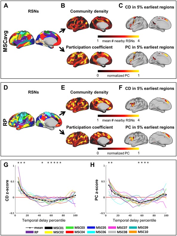
Early regions preferentially localize to areas proximal to multiple functional systems. (A) RSN parcellation computed from the MSC average correlation matrix, as previously published (Gordon et al. 2017c), provided for reference. (B) Upper: Community density map for the MSC average, averaged across correlation thresholds or “edge densities” (see Methods). Higher values indicate proximity to a greater number of RSNs. Lower: Participation coefficient map for the MSC average, averaged across correlation thresholds. (C) Upper: MSC average community density (upper) and participation coefficient (lower) maps in (B), thresholded by the earliest 5% of vertices in the MSC average weighted lag projection (shown in Fig. 1). (D–F) Same as (A–C), but for the individual subject RP. RP RSN parcellation, provided for reference, is from Laumann et al. (Laumann et al. 2015). (G) Standardized community density, for each individual, as a function of increasing latency. Black opaque curve represents average curve across individuals. Community density was averaged into 5% bins spanning the range of lag projection values, ordered from early-to-late. One-sample t-tests determined, for a given latency bin, mean community density across individuals that differed from the expected value. (*P < 0.05 following Bonferroni correction for 20 bins). (H) Similar analysis as in (G), but for participation coefficient instead of community density.
Lag Analysis
The Pearson correlation coefficient,  , for zero-lag correlation between continuous signals,
  and
and  , is given by:
 |
(1) |
where  and
and  are the temporal standard deviations of the zero-mean signals
  and
and  and
and  is the interval of integration. By generalizing this equation to accommodate temporal delays,
  , between the signals, correlation (or covariance, for simplicity) can be computed as a function of delay in seconds. Thus,
 |
(2) |
defines the CCF. The lag between  and
and  ,
,  , is then determined to be the value of
  at which
  exhibits an extremum. Thus,
 |
(3) |
While the CCF of periodic time series is likely to feature multiple extrema, BOLD signals are aperiodic (He et al. 2010) and almost always produce a single, well-defined cross-covariance extremum for a given pair of time series, typically in the range of ±1 s.
In practice, we first construct the CCF in the time domain at discrete multiples of the TR (i.e., at the sampling interval) (see Raut et al. 2019 for a more detailed explanation). A single CCF for each session is obtained by summing unnormalized cross-covariance over blocks ( ) of contiguous frames, and subsequently normalizing based on the total number of time points in a session contributing to a given CCF lag. Thus,
 |
(4) |
 |
(5) |
where  is the temporal shift in units of TRs,
  indexes frames within the block,
  is the total number of frames within the block,
  is the total number of frames contributing to the CCF estimate at a particular temporal shift, and
  is the total number of blocks. Time series are set to zero-mean prior to Equation (4) by subtracting the mean computed over the maximum number of realizations (i.e., all non-censored frames from the time series).
We used three-point parabolic interpolation centered on the empirical peak of  (and the immediately preceding and succeeding samples) to approximate the extremum and its associated abscissa,
  at a temporal resolution finer than the sampling rate. Time delays longer than 4 s (
 = 4 s) were discounted as, in our experience, such results appear to reflect sampling error or artifact.
  was computed over
 [−4, 4] and [−3, 3] for RP (TR = 1.16 s) and MSC (TR = 2.2 s), respectively. Performing minimal time shifts reduces the minimum duration required for a block of contiguous frames to contribute to each point of the CCF, which maximizes data usage (Raut et al. 2019).
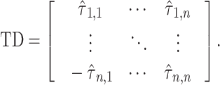
The above approach can be generalized to a set of  time series
  . Thus,
  will be an
  cross-covariance matrix from which
  can be obtained for every pair of time series,
  , yielding an
  time delay matrix:
 |
(6) |
The diagonal entries of  are 0 by definition, because any time series is perfectly correlated with itself at zero-lag. Moreover,
  is anti-symmetric (
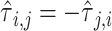 ): if the time series
  is determined to precede
  by a certain magnitude, then
  can equivalently be said to succeed
  by the same magnitude, yielding the opposite sign.
Here we compute  as the temporal delay of
  relative to
  , such that a negative value implies that
  precedes
  . Thus, following Nikolic et al. (Schneider et al. 2006; Nikolić 2007), a column-wise mean yields a one-dimensional projection of
  , which we refer to as a “lag projection” (
 ), which reflects the mean latency of each vertex with respect to all other vertices. Thus,
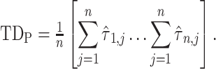 |
(7) |
Further, for a given “seed” region comprising one or multiple vertices, the entire rows of  corresponding to these vertices can be averaged to give a seed-based lag map—a one-dimensional map of each vertex’s temporal delay with respect to the seed.
Pairwise TD root mean square error is inversely related to zero-lag correlation magnitude,  . We have previously modeled this relationship as follows:
 |
(8) |
where  is fit by conventional regression (Raut et al. 2019). This relation can be used to reduce lag projection sampling error by down-weighting high-variance lag estimates. Thus, we additionally computed weighted lag projections (
 ) by inversely weighting TD pairs in proportion to modeled squared error. Thus,
 |
(9) |
Importantly, values in weighted lag projections—as in unweighted lag projections—retain the dimension of time and are therefore expressed in seconds.
MATLAB code for computing lag analyses as described in this paper is publicly available at https://github.com/RaichleLab/lag-code .
Similarity Analysis
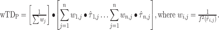
Similarity of surface maps (Figs. 3 and 4) was computed as the Pearson spatial correlation over vertices. For TD and FC matrices, this measure was computed over the vectorized upper triangular of the full 7320 × 7320 matrix. Statistical significance of differences in similarity (Fig. 3) was assessed with Student’s paired t-tests performed on the Fisher-z transformed r values. For comparisons involving the MSC average, the MSC average was computed using all 100 sessions.
Figure 3.
Specificity and reliability of BOLD spatiotemporal structure in individuals. (A) Split-half similarity matrices computed for TD matrices from each of the MSC subjects and RP. Each element in these matrices is a Pearson correlation coefficient between half of one subject’s data and half of another (or the other half of the same) subject’s data. The final row/column reflects correlations with the MSCavg. The left panel includes all time delays (i.e., the full TD matrix). In the middle panel, time delays corresponding to region pairs with zero-lag correlation magnitude <0.2 (as determined by the MSCavg) are excluded from the similarity computation. Excluding unstable time delays in this way improves within- (on-diagonal) and inter-individual (off-diagonal) correspondence and makes individual-specificity more apparent (comparison of on-diagonal blocks versus the final row/column). Reliability and individual-specificity are further augmented by increasing the correlation threshold to 0.4 (right). (B) Split-half similarity matrices for lag projections—both unweighted (left) and weighted (right) column-wise means of time delay matrices, where weighting is with respect to zero-lag correlation magnitude. Lag projections, particularly when weighted, are relatively stable measures of latency structure and also exhibit individual-specificity. (C) Split-half similarity matrix for the full FC matrix from each subject, which is more stable than measures of latency structure. (D) Summary and comparison of intra-individual (red), inter-individual (blue) and individual-to-group (black) similarity for different spatiotemporal measures, represented as Fisher z-transformed correlation coefficients. Intra-individual, inter-individual, and individual-to-group similarity were separately compared for both TD matrices computed across the different FC thresholds and for unweighted and weighted lag projections. Statistical significance was assessed by two-tailed paired t-tests (N = 11; ***P < 0.001; n.s., not significant).
Figure 4.

Data requirements for different measures of BOLD spatiotemporal structure. (A) Example TD matrices and weighted lag projections computed from two randomly split halves of RP’s data. Rows and columns of the first half TD matrix have been sorted from early-to-late, and by network affiliation following (Laumann et al. 2015). Half 1 sorting was applied to the TD matrix from Half 2. Note largely orthogonal relationship of latency structure to RSNs manifesting as a wide range of TD values within matrix blocks (Mitra et al. 2014). Also note that early (late) regions tend to be early (late) in both within- (on-diagonal) and between-RSN (off-diagonal) relationships (Mitra and Raichle 2018). (B) Correlation of spatiotemporal structure from one half of RP’s data with the spatiotemporal structure computed from increasing amounts of data drawn from the other half. Correlation is computed for several measures of spatiotemporal structure: full TD matrix (pink), TD matrix excluding |FC| < 0.2 (orange), TD matrix excluding |FC| < 0.4 (red), unweighted lag projection (blue), weighted lag projection (black), and the full FC matrix (green). For FC-based thresholding, FC is determined by the FC matrix computed over all RP data. Correlation curves are represented as mean (solid line) and SD (shaded surrounding area) of correlation from 100 random samplings of the 88 ten-min sessions.
Community Detection and Graph Analyses
Individual-specific RSN parcellations were computed by subjecting weighted graphs, constructed from thresholded vertex-wise correlation matrices (suprathreshold values retained), to the InfoMap community detection algorithm (Rosvall and Bergstrom 2008), as in prior descriptions of RSN organization in the present individuals (Laumann et al. 2015; Gordon et al. 2017c). Community density maps were computed following Power et al. (Power et al. 2013). Specifically, for each cortical vertex (at ~2 mm resolution, ~32 k vertices per hemisphere) and each correlation threshold (i.e., thresholds retaining the top 0.5–2.5% of correlations, in 0.5% steps) we computed the number of unique communities present within a given radius of the vertex center. Radii of 5–10 mm in 1 mm steps were analyzed, and community density maps were averaged across the five correlation thresholds. Hence, 30 total analyses (five thresholds x six radii) contributed to the mean community density map of each individual.
Participation coefficient,  , was computed for each node,
  , following Guimerà & Nunes Amaral (Guimerà and Nunes Amaral 2005); thus,
 |
(10) |
where  is the sum of supra-threshold correlations (i.e., sum of “weighted edges”) of node
  to nodes in module
  , and
, and  is the sum of all supra-threshold correlations of
  . Greater values of
  therefore indicate increasingly uniform distribution of strong correlations among all modules. To reduce computational demand, participation coefficient was computed using the same 6 mm resolution vertices that formed the ROIs for lag analyses. Participation coefficient was analyzed across 10 correlation thresholds that achieved a similar range of graph sparsity to those used for community density analyses; these were the top 10–2% (in 0.5% steps) of correlations (Power et al. 2013). Participation coefficient values were subsequently summed across thresholds and normalized relative to the maximum possible value (i.e., 10), and up-sampled to 2 mm resolution to match community density.
For inter-subject comparison, graph metrics were first standardized (zero-meaned and given unit standard deviation) within each individual. Standardized community density values were subsequently averaged into 5% bins spanning the range of lag projection values, ordered from early-to-late. Mean correlation magnitude (“node strength” in graph terms) was computed as a row-wise sum of the absolute value correlation matrix and similarly standardized within-individual and analyzed across different percentile bins of the up-sampled lag projection.
Statistical significance of community detection, participation coefficient and node strength values for each lag percentile bin was determined by one-sample t-tests against the null hypothesis of Z-score = 0 (Bonferroni correction for 20 bins).
Results
Individual-specific Patterns in Brain-wide Latency Structure
We examined individual-level BOLD lag structure in the recently published “MyConnectome” (Laumann et al. 2015; Poldrack et al. 2015) and “Midnight Scan Club (MSC)” (Gordon et al. 2017c) datasets. These datasets comprise, respectively, 88 ten-min scans in one individual (initials R.P.) and 10 thirty-min scans in each of 10 individuals (100 scans in total).
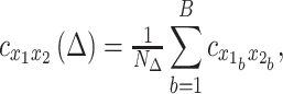
Temporal sequences of ISA can be studied by computing interregional time delays in the BOLD signal. Here, we determine lag as the time shift that optimizes the covariance between a given pair of time series; we use parabolic interpolation of the cross-covariance curve to resolve time delays finer than the sampling rate (see Methods). All pairwise delays are assembled into an anti-symmetric time delay (TD) matrix. Despite high-dimensionality (Mitra et al. 2015a), BOLD TD matrices are significantly transitive (Mitra et al. 2014). Thus, there exists a dominant propagation pattern that can be represented as a one-dimensional brain map, computed as the column-wise mean of the TD matrix (Schneider et al. 2006). The resultant “lag projection” reflects each region’s mean temporal lead or lag relative to all other regions. Computing the projection as a weighted column-wise mean, where weight is inverse to TD variance (see Methods), improves the reliability of the estimate (Raut et al. 2019).
Figure 1A illustrates weighted lag projections averaged across all MSC subjects (henceforth referred to as the group average) and the individual, RP. Bilaterally symmetric, distributed “early” and “late” regions are immediately apparent in both the group and individual. Figure 1B extends this result to each of the MSC individuals. Importantly, the topography of early and late regions varies from subject to subject yet is generally similar across individuals. Thus, BOLD temporal lag structure is robust at the individual level, although some features of this structure exhibit individual variations, which we discuss further below.
Figure 1.

Individual and group patterns of latency structure. (A) Weighted lag projection maps from data averaged over individuals (MSCavg; left) and from one separate individual, “RP” (right). Weighted lag projections are one-dimensional representations of latency structure computed as a column-wise weighted mean of the time delay matrix. More strongly correlated regions are given greater time delay weights (see Methods). (B) Weighted lag projection maps for each of the MSC subjects. Note larger lag projection values in individual as compared to MSC averaged results, likely attributable to inter-subject variability in the latter.
Spatiotemporal Structure within Conventional Functional Networks
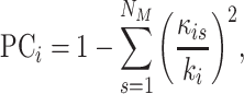
Prior findings have demonstrated that lag structure is largely orthogonal to conventional RSN boundaries (Mitra et al. 2014). Thus, rather than functionally-related regions being iso-latent, temporal delays on the order of 1 s are apparent within each major large-scale network. In other words, no network is wholly either early or late, provided the analysis is conducted in awake subjects (Mitra et al. 2015b). To explore this property in the individual, we computed seed-based lag maps in two large, distributed networks. Seeds were placed in the dorsolateral prefrontal cortex (Fig. 2A), which largely corresponds to the frontoparietal control network (FPC) (Dosenbach et al. 2007; Vincent et al. 2008), and the precuneus (Fig. 2B), a hub of the default mode network (DMN) (Greicius et al. 2003). These maps reflect latency of each region with respect to the seed. As is evident in Figure 2, these networks exhibit a range of delays on the order of 1 s in both the MSC average and individual. Moreover, several spatiotemporal features within these networks are common to the group. For instance, in the FPC, a lateral prefrontal early-to-late gradient in the posterior-to-anterior direction is prominent in both the group and each individual, in addition to an early region in the dorsomedial prefrontal cortex. In the DMN, early-to-late gradients are present in the precuneus, the earliest region being the retrosplenial cortex. On the other hand, the medial prefrontal cortex, while late in the group average, is not appreciably later than the rest of the DMN in one individual, RP. In sum, even at the individual level, BOLD fluctuations are not temporally synchronous within RSNs. Moreover, individual variability in latency structure can exist even where RSN spatial topography, defined by zero-lag FC, is largely conserved.
Figure 2.
Spatiotemporal structure of RSNs shows similarities and differences between the group and individual. Seed-based lag maps reflect each vertex’s lag with respect to the seed region. Seeds were placed in the dorsolateral prefrontal cortex (A) and precuneus (B) (white circles outlined in black). Maps are thresholded at zero-lag correlation r > 0.2. (A) The group average (left) and an individual, RP (right) show similar lagged relationships across distributed regions of the frontoparietal control network. (B) The group (left) and RP (right) also exhibit similar spatiotemporal features within the default mode network; however, the medial prefrontal cortex (pink arrow) is a notable exception.
Specificity and Reliability of Latency Structure in Individuals
Given the presence of such individual differences, the question arises as to whether these differences stem primarily from sampling variability or true individual-specific spatiotemporal patterns in spontaneous activity (or other potential sources unrelated to sampling variability, such as registration errors). We addressed this question by dividing the total number of sessions available for each subject into random split halves and computing spatial correlations between measures obtained from each of these halves (within and between subjects). Thus, we defined similarity (or, in the case of intra-individual comparison, “reliability”) as the Pearson correlation coefficient between two halves. Each half comprises 150 min of data for MSC subjects and 440 min of data in RP.
Figure 3 displays the resulting split-half similarity matrices for several measures of spatiotemporal structure, where diagonal two-by-two blocks correspond to intra-individual correlation, off-diagonal blocks reflect inter-individual correlations, and the final row and column reflect correspondence with the MSC average. Figure 3A reflects the subject-specificity and reliability of TD matrices. For MSC subjects, intra-individual reliability of the full TD matrix is notably weak and is generally lower than correlation with the group, which comprises 3000 min of data (Fig. 3A, left). This result is expected given the sensitivity of BOLD TD estimation to sampling variability, particularly among pairs of weakly correlated time series, which constitute the majority of time series pairs in global signal regressed-data (Raut et al. 2019).
If sampling variability is the primary explanation for low intra-individual reliability, focusing on more strongly correlated time series should improve reliability. Indeed, by excluding time series pairs with correlation magnitude below 0.2 or 0.4 (Fig. 3A middle and right, respectively), as determined by the group average FC matrix, intra- and inter-individual similarity of time delay relationships are markedly improved for all subjects. Importantly, intra-individual similarity (near-diagonal blocks) exceeds similarity to the group average (last row/column) when excluding weakly correlated region pairs. Thus, sampling variability obscures true individual differences in latency structure. This inference is further supported by the fact that RP exhibits moderate reliability even across the full TD matrix, and in general exhibits much greater reliability than the MSC subjects, each of whom have less than half the data quantity of RP. Split-half similarity of lag projections (Fig. 3B), which are more stable representations of latency structure, further supports the existence of stable individual-specific features in latency structure. For comparison, Figure 3C shows a similarity matrix for FC computed from the same data; lag and FC similarity results are summarized in Figure 3D.
Note that for all comparisons involving the MSC average, the MSC average was computed using all 100 sessions in order to maintain a consistent comparator. In practice, removing the split-half of interest from the MSC average before computing similarity yields comparable results (z(r) values in Figure 3D corresponding to correlation with MSCavg are decreased by (mean ± standard deviation) 0.122 ± 0.008 for the “all pairs” TD condition, 0.021 ± 0.007 for lag projections, and 0.007 ± 0.002 for FC after removal).
Findings thus far point to sampling variability as the primary obstacle to studying latency structure in individuals. To answer the question of how much data is needed to resolve measures of BOLD spatiotemporal structure in individuals, we computed the spatial correlation between measures generated from one half of RP’s data with increasing quantities of the other half, as done previously for FC (Laumann et al. 2015). Results are displayed in Figure 4. These plots show that a substantial quantity of data is required to stabilize the full TD matrix, which includes TD estimates between many weakly correlated region pairs. Restricting the analysis to moderately correlated region pairs can dramatically decrease data requirements. Further, weighted lag projection maps at 6 mm-resolution can achieve a correlation of 0.8 with ~25 min of data. FC matrices, as discussed above, are more stable than each of these measures of latency structure. Importantly, it should be noted that reliability in RP is limited by known systematic differences in the state of the subject across different scanning days (e.g., fed vs. fasted and caffeinated vs. non-caffeinated; see Methods) (Laumann et al. 2015; Poldrack et al. 2015), which are associated with differences in latency structure (Fig. S1).
Patterns of Intra- and Inter-individual Variability
To further investigate factors affecting intra- and inter-individual consistency of latency structure, we computed the standard deviation of each TD pair (TDstd) across sessions (within each subject) and across subjects (averaged across sessions). We examined regional patterns of variation along these two dimensions by computing the mean TDstd at each vertex; these patterns are displayed in Figure 5. Given the low reliability of lag estimates derived from single sessions, intra-individual variability may be expected to reflect sampling error rather than true day-to-day variance in neural activity. Indeed, we found that the spatial topography of observed intra-individual variability in latency structure can be largely predicted by the regional topography of mean FC magnitude (r = −0.91; Fig. 5A, lower). Thus, because TD sampling variability is inversely related to correlation magnitude (Raut et al. 2019), regions that are strongly correlated (or anti-correlated) with large portions of the brain—such as regions in the default mode network—tend to show less variability in lag estimates across sessions. Despite 30-min sessions in MSC subjects, mean TD standard deviation across sessions and mean FC magnitude were still strongly negatively correlated across the brain (r = −0.93 ± 0.02 for MSC subjects). Importantly, this topography relating to FC magnitude is distinct from the topography of intra-individual variability in FC, which is most apparent in motor and visual areas (Laumann et al. 2015).
Figure 5.
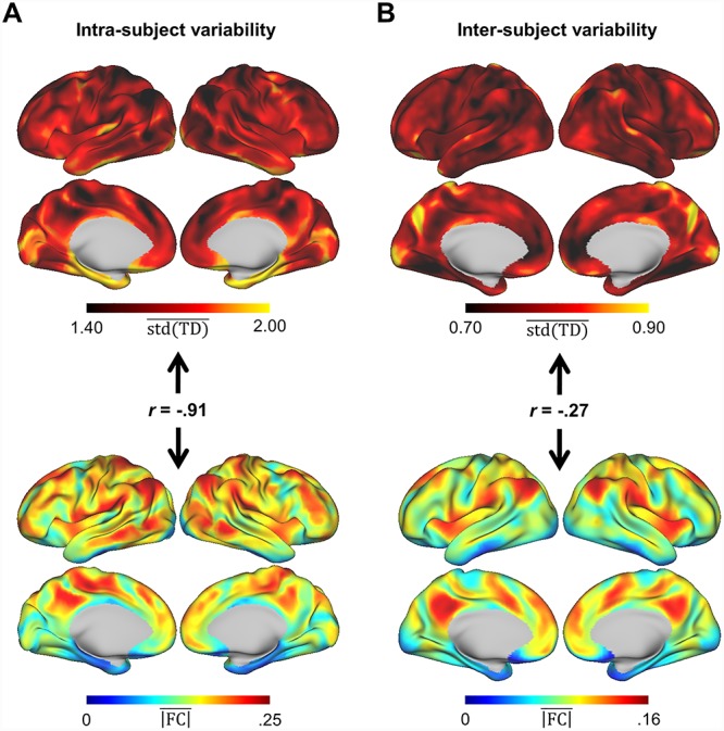
Regional patterns of variability in latency structure. (A) Upper: Map for RP reflecting, for each vertex, TD standard deviation (TDstd) across sessions and subsequently averaged across all of the vertex’s TD relationships (column-wise mean of TDstd). Lower: Each vertex’s mean zero-lag correlation magnitude. The strong inverse correlation between these maps (r = −0.91) implies that regions that exhibit the most session-to-session TD variability tend to have weaker correlations in general, making their TD relationships more prone to sampling variability. (B) Upper: Map reflecting column-wise mean of TDstd, as in (A), but where TDstd is computed across all MSC subjects rather than RP sessions. Lower: Each vertex’s mean zero-lag correlation magnitude, computed from the MSC average. Despite 300 min of data per subject, there is still contribution of sampling variability (r = −0.27 between upper and lower maps). However other sources of variability, such as anatomical, are now apparent.
To examine inter-individual variability, we used the full 300 min of data obtained in each MSC subject. Regional inter-individual variability is shown in Figure 5B. While this pattern is still inversely correlated with mean FC magnitude as determined by the MSC average (r = −0.27), sources of variability other than sampling error now are prominent. One such source is likely anatomical variability—as seen, for example, at the temporoparietal junction (Mueller et al. 2013). Anatomic variability may, in part, reflect imperfect registration of individuals to the fs_LR atlas surface (Van Essen et al. 2012). The map of inter-individual TD variability also bears some resemblance to that of inter-individual FC variability, as both feature high values in temporoparietal junction, dorsolateral prefrontal cortex, and lateral visual areas (Mueller et al. 2013; Laumann et al. 2015). Regions of high variability in lag and correlation structure may reflect, to varying degrees, individual differences in anatomy or functional organization.
Consistent Features of Latency Structure Across Individuals
Despite robust individual differences, it is evident from Figure 1 that many features of latency structure are similar across subjects. To determine the consistency in location of early and late regions, we computed spatial overlap by summing, across individuals, binarized maps reflecting the earliest 15% and latest 15% of vertices in each individual’s lag projection. These overlap maps are shown in Figure 6. Early regions exhibit a high degree of overlap, with multiple regions present in all 11 subjects. Regions that tend to be among the earliest across subjects localize to inferior frontal gyrus, lateral premotor cortex, frontal eye fields, dorsal anterior cingulate/pre-supplementary motor area, and retrosplenial cortex, as well as the left anterior insula. The majority of these regions are recruited across a wide range of behavioral paradigms studied with task-based fMRI (Dosenbach et al. 2006; Duncan 2010; Nelson et al. 2010; Yeo et al. 2015); the significance of this correspondence is considered in the Discussion. Late regions show substantially less overlap across subjects but include visual cortex, the inferior temporal gyrus, and orbitofrontal cortex.
Consistent Relationships Between Latency Structure and Correlation Structure
Notably, the highly consistent early regions shown in Figure 7 are not all associated with the same functional network. This is in agreement with prior findings indicating that conventional RSNs each comprise early and late regions separated by ~1 s (Mitra et al. 2014) (also see seed-based lag maps in Fig. 2 and time delay matrix in Fig. 4). In principle, each network may have its own early and late regions; alternatively, a smaller set of early and late regions may span multiple networks. Visual inspection of Figure 7 suggests the latter possibility: early regions in particular tend to avoid the large patches of cortex associated with single functional systems, and instead are positioned near the boundaries of multiple RSNs. For example, consistent early regions are absent from most of sensorimotor cortex but localize focally to the caudal portion of dorsolateral prefrontal cortex, which overlaps premotor and attentional areas in addition to the ventral motor strip (Fig. 6). Likewise, the DMN is largely devoid of early regions save for the retrosplenial cortex (Mitra and Raichle 2018), which is proximal to extrastriate visual cortex and areas related to the processing of contextual, visuospatial information (Bar and Aminoff 2003; Gilmore et al. 2016). Thus, early regions appear to fall largely within previously reported zones of high “community density (CD),” or cortical regions where multiple RSNs are in close spatial proximity (Power et al. 2013).
To quantitatively assess the relationship between temporal latency and RSN proximity, we computed CD as done previously (Power et al. 2013). Thus, putative RSNs were first identified in each subject by applying a commonly used community detection algorithm to the thresholded zero-lag correlation matrix (Rosvall and Bergstrom 2008; Power et al. 2011). At each vertex, the number of nearby communities (RSNs) was averaged across a range of correlation thresholds (edge densities), accounting for the inherently hierarchical organization of RSNs. Figure 7B displays an example CD map computed from the MSC average correlation matrix. Thresholding this map by a mask of the earliest 5% of regions in the MSC average weighted lag projection reveals relatively high values of CD (Fig. 7C). Figure 7D–F displays similar results for the individual, RP. In each individual we computed the mean CD value within progressively later 5% bins of the latency-sorted weighted lag projection. The resulting CD curves as a function of increasing latency are displayed in Figure 7G, which demonstrates, in each individual, a clear bias for early regions to localize to zones of high CD (P < 0.05, Bonferroni correction for 20 bins). Regions that are neither very early nor late tend to exist in regions with significantly below-average CD. Interestingly, this bias toward low CD regions is not present for the latest regions.
The above described finding suggests that the activity of early regions may be associated with that of multiple networks, rather than strongly associated with a single network. To test this, we repeated the above analysis, replacing CD with the graph metric of participation coefficient (PC) (Guimerà and Nunes Amaral 2005), as computed previously for fMRI correlations (Power et al. 2013) (eq. 10). PC quantifies the extent to which the associations of a node (here, the strongest correlations of a vertex) are distributed uniformly among communities (RSNs). Results displayed in Figure 7H confirm that early regions in each individual exhibit strong correlations more uniformly distributed among RSNs, and progressively later regions show significantly below-average PC values (with no consistent lag: PC relationship for the latest regions) (P < 0.05, Bonferroni correction). Conventional interpretation of high PC is that such nodes are vital for connecting distributed communities (Bertolero et al. 2017); however such an interpretation is at least partially confounded in BOLD data by spatial autocorrelation. Thus, although this result confirms that the time series of early regions exhibit characteristics of multiple, rather than single RSNs, high PC does not necessarily imply a relationship with multiple networks beyond spatial proximity.
Regions with near-zero lag projection values are preferentially localized to low CD (and low PC) regions; in theory, this may be a trivial result of near-zero-lag regions being less widely correlated with the rest of the brain. That is, regions that do not have robust relationships with most of the brain may be less likely to be very early or late as indicated by the lag projection map, which reflects each region’s mean temporal relationship with respect to all other regions in the brain (although this scenario is less likely for correlation-weighted lag projections, as used here). To test this possibility, we repeated the above analyses with “node strength,” computed for each vertex as the sum over rows of the absolute value FC matrix. None of the 20 latency bins exhibited node strength values that significantly deviated from the mean (P > 0.05, Bonferroni correction). Thus, the preferential location of apparent cortical “source” regions proximal to multiple RSNs, as well as their shared signal with multiple networks, is not explained by a confounding relationship between lag projection values and correlation magnitude.
It is also conceivable that long-latency regions appear less strongly associated with single networks simply because network structure is defined here on the basis of the zero-lag correlation matrix, rather than a correlation matrix that accounts for temporal delays (peak-lag correlation matrix). For this to be true, the zero-lag and peak-lag correlations should materially differ. Importantly, this is not the case for BOLD time series (which are essentially restricted to frequencies below 0.1 Hz) within the range of lags studied here (± 4 s). To empirically verify, we computed, for each of the 100 sessions comprising the MSC dataset, the correlation coefficient between the (Fisher z-transformed, upper triangular) zero-lag and peak-lag correlation matrices. This value exceeded 0.99 in all 100 sessions (mean ± standard deviation = 0.9963 ± 0.0014; range = [0.9921, 0.9983]). Thus, network construction from zero-lag, rather than peak-lag correlations does not account for the tendency of near-zero-latency regions to correlate more strongly with—or exist well within the bounds of—single functional networks.
Discussion
The analysis of resting-state fMRI has been largely focused on zero-lag FC, computed either using Pearson correlation (Biswal et al. 1995) or spatial independent component analysis (Beckmann et al. 2005). Nevertheless, large-scale propagation dynamics in resting-state fMRI have also been studied using a variety of analytic approaches (Sun et al. 2005; Garg et al. 2011; Majeed et al. 2011; Friston et al. 2013; Friston et al. 2014; Gilson et al. 2016; Schwab et al. 2018; Casorso et al. 2019). These studies have provided compelling evidence of spatiotemporal dynamics in BOLD time series not captured by zero-lag correlation (Liégeois et al. 2017). Here, we demonstrate that widespread latency structure revealed by pairwise cross-correlation generally is consistent across individuals. At the same time, statistically reliable individual differences also are present. Inter-regional lag relationships in resting-state fMRI are not predicted by zero-lag correlation (Mitra et al. 2015a). Thus, in addition to the spatial organization of BOLD fluctuations described by zero-lag correlation structure, temporal latency structure represents another fundamental organizational property of BOLD signals. The study of individual-specific organization in intrinsic brain activity, as well its relation to behavior or pathology, may therefore benefit from the analysis of BOLD time delays.
Robustness of Temporal Latency Structure Within Individuals
To date, studying brain-wide temporal latency structure has made use of large datasets in order to overcome sampling variability, leaving undetermined the extent to which such structure is apparent at the individual level. The present finding of reproducible temporal latency structure in highly-sampled individuals suggests that, like correlation structure, this temporal structure is a fundamental mode of organization present in spontaneous brain activity. As is apparent in large group averages (Mitra et al. 2014), we find that temporal latency structure is largely orthogonal to functional networks (Figs. 1 and 4), with a range of delays apparent both within and between networks. One apparent exception to this observation is the relatively uniform precedence of activity in the visual network relative to the somatomotor network seen in RP (Fig. 4); this is likely attributable to RP being scanned in the eyes-closed state, which has previously been shown to increase relative earliness of resting-state BOLD signals in visual cortex (Mitra et al. 2014). Along with latency changes related to caffeine and food consumption (Fig. S1), these differences highlight the sensitivity of BOLD latency structure to arousal and neuromodulation. Given these state differences, it is likely that true day-to-day variance in neural latency structure also contributes to inter-session variability, although this source of variability would be dominated by sampling error in conventional data quantities (Raut et al. 2019).
Implications of Reproducible Individual Differences in Latency Structure
There is growing interest in and appreciation for individual differences in the spatial organization of functional networks, as studied with rsfMRI (Mueller et al. 2013; Laumann et al. 2015; Braga and Buckner 2017; Gordon et al. 2017c; Gratton et al. 2018; Kong et al., 2018; Marek et al. 2018). The presence of individually-specific patterns of latency, particularly in the context of common zero-lag correlation structure (Fig. 2), adds an additional level of complexity to the organization of spontaneous infra-slow activity in the human brain. For example, to the extent that infra-slow activity reflects a form of large-scale neural communication, the present findings suggest that individuals may differ not only in which regions tend to be engaged simultaneously, but how, in terms of the direction of signaling, this communication tends to take place. The source of such individual differences in directed propagation currently is unclear. We have previously shown that behavior can alter resting-state latency structure (Mitra et al. 2014); thus, as has been hypothesized for FC (Harmelech and Malach 2013), plastic changes over time may lead to individual-specific biases in the propagation of spontaneous brain activity. Nonetheless, it is difficult to separate variability in lag relationships from spatial variability in functional organization that is present at a range of spatial scales. Although not the focus of the present work, future analyses may attempt to account for some such spatial variability in functional topography (e.g., Guntupalli et al. 2018) prior to lag analysis. Incorporation of behavioral, task-evoked or structural data will also likely aid interpretation of individual variability in latency structure.
Studying Latency Structure in Individuals
Given sufficient data, a largely preserved temporal structure of spontaneous infra-slow activity is observable in individual humans, along with highly reproducible individual-specific features (Figs. 1 and 2). However, despite the relatively large amount of data collected in each of these individuals compared to standard ~10-min acquisitions, some aspects of latency structure remain subject to significant sampling variability, even in the highly sampled MSC subjects, each with 300 min of data.
For a given data quantity, variance in latency structure is largely determined by the strength of correlation (Raut et al. 2019). This relationship is evident in Figures 3 and 4, in which reliability (and stable individual-specific features) is progressively enhanced by excluding weakly correlated relationships. On the other hand, the relationship between correlation and lag variance may not always be obvious, and failure to appreciate this relationship can lead to misinterpretation of findings. For example, Figure 5A (upper) displays inter-session (intra-subject) TD variance, which may be mistaken for neural day-to-day variability in temporal relationships. However, by computing a regional map of mean correlation magnitude (Fig. 5A, lower), we demonstrate that this variability is largely attributable to sampling error associated with estimating lag between weakly correlated signals. Thus, it is crucial to consider sampling variability when studying lag structure, particularly in relatively small datasets such as those collected in individuals.
How, then, may individual differences in latency structure be probed? The necessity of acquiring atypically large quantities of data to properly characterize individual-specific patterns of FC is increasingly recognized (Laumann et al. 2015; Gordon et al. 2017c). Datasets from highly-sampled individuals are likely to provide opportunities to study more stable features of latency structure, such as lag projections and lags between strongly correlated regions (e.g., intra-network lags). How much data is needed? We address this question in Figure 4. Weighted lag projections can achieve good reliability (r > 0.9) with 100 min of data—less than a third of the data available for MSC subjects. In practice, precise data quantities required for estimating spatiotemporal structure will depend on the resolution of the analysis (e.g., vertex/voxel-level versus region-level) as well as pre-processing choices (e.g., degree of spatial smoothing and nuisance regression).
Functional Significance of Consistent Early Regions and Their Proximity to Multiple RSNs
Despite the presence of fine-scale individual-specific patterns, latency structure was generally similar across individuals. Indeed, despite relatively low inter-individual similarity at the voxel/vertex level, similarity of individual latency structure with the group average was substantial (Fig. 3). By examining mean latency of each region relative to the rest of the brain (lag projection), we identified a relatively sparse, focal set of very early regions present in most or all 11 individuals studied here (Fig. 6). Interestingly, topographic correspondence was much more consistent for early regions than late regions. This suggests that the cortex contains multiple spatially constrained generators of infra-slow fluctuations, the propagation of which may be diffuse or distributed. Importantly, the lag projection represents a likely superposition of multiple spatiotemporal processes (Mitra et al. 2015a). Thus, early regions are not likely to act as distributed generators of a single, brain-wide infra-slow process, but may instead be associated with distinct widespread phenomena.
Consistently early regions included lateral premotor areas, the inferior frontal gyrus, the dorsal anterior cingulate/pre-supplementary motor area, and anterior insula—all of which belong to a previously described “multiple-demand system” (Duncan 2010) comprising regions that exhibit task-related activity across a wide range of behavioral paradigms (Dosenbach et al. 2006; Nelson et al. 2010; Hugdahl et al. 2015; Yeo et al. 2015). In addition to these regions, we also identified the retrosplenial cortex as a consistently early region of the default mode network. Finally, we find the left anterior insula to be asymmetrically early, despite all other early regions being bilaterally symmetric. Interestingly, functional asymmetry in this region has been widely observed (Craig 2009) and has been previously interpreted in the context of parasympathetic and sympathetic afferents to the left and right insula, respectively (Craig 2005).
In addition to this behavioral relevance, we identify a bias in the localization of cortical infra-slow sources in relation to known functional systems. Each canonical RSN exhibits a range of temporal delays (e.g., Figs. 2 and 4) (Mitra et al. 2014); this suggests that the earliest regions of cortex may be expected to be distributed among RSNs. Here, we find that cortical source regions are further constrained by their preferential location proximal to multiple networks. Several of these high community density regions are small patches of cortex that are functionally well-defined (e.g., anterior insula, frontal eye field) yet are surrounded by regions associated with varying functional systems. Considering their correspondence with several regions commonly recruited by tasks, we suggest that these regions share an ability to broadly influence cortical excitability. That is, these regions may have, at least in theory, high “average controllability” over widespread brain activity (Muldoon et al. 2016). Such an interpretation is consistent with early regions additionally exhibiting high participation coefficient. Several studies have applied this graph metric to fMRI data in order to identify putative hubs supporting integration among RSNs (e.g., Power et al. 2013; Bertolero et al. 2015; Shine et al. 2016; Bertolero et al. 2017; Hwang et al. 2017; Gordon et al. 2018). Note, however, that due to spatial autocorrelation in BOLD data, this metric may conflate to some degree true hub-like properties with those reflected in community density (i.e., spatial proximity to multiple functionally distinct regions).
Notably, task-evoked infra-slow responses in the early regions identified here have also been shown to be relatively early compared to the responses of other regions involved in the same tasks (Goebel et al. 2003; Sun et al. 2005; Sridharan et al. 2007; Bressler et al. 2008; Sridharan et al. 2008; Kayser et al. 2009; Foster et al. 2012; Asemi et al. 2015; Spadone et al. 2015). Thus, broad influence of early task regions may also be continuously exerted in spontaneous brain activity, or their earliness observed here may be pertinent to ongoing behavior in the “resting-state.” Additionally, the proximity of early regions to diverse RSNs may confer privileged influence over the excitability of disparate functional systems (e.g., the unique position of retrosplenial cortex adjacent to visual cortex, the medial temporal lobe, and the DMN, all of which share reciprocal connections with this region (Vann et al. 2009)). Retrosplenial cortex in particular was also found to exhibit early, high-amplitude BOLD transients relative to other cortical regions in association with hippocampal sharp-wave ripple events (Ramirez-Villegas et al. 2015); thus, earliness in retrosplenial cortex may result from this region being an early cortical target of ripples, or alternatively, is a general feature that is relevant for both cortico-cortical and hippocampal-cortical communication. Finally, it is plausible that cortical infra-slow sources share a unifying biological quality—such as affinity for a particular neuromodulator or high density of afferents from a certain subcortical population—that explains their temporal characteristics, although this remains to be investigated. In any case, BOLD fluctuations appear to propagate from regions of high community density into major RSNs, as corroborated by the tendency for regions of below-average community density (i.e., those deep within a single major RSN) to be closer to zero-latency in the lag projection.
When interpreting temporal relationships among fMRI signals, it must be appreciated that BOLD time delays specifically reflect the propagation of infra-slow brain activity (Mitra et al. 2018). We have previously provided evidence for infra-slow propagation in what might be considered a “feedback” direction, or from the “recipient” to the “sender” of the higher-frequency activity that may carry feed-forward information (Mitra et al. 2016). Using wide-field imaging we have observed that roughly reciprocal directions of propagation between infra-slow and delta (1–4 Hz) activity extend across mouse cortex (Mitra et al. 2018). The hypothesized tendency of infra-slow source regions to initiate widespread changes in cortical excitability may serve to coordinate—perhaps through phase-amplitude coupling (Monto et al. 2008; Canolty and Knight 2010; Mitra et al. 2018)—incoming information from widespread regions that is carried in higher frequencies (Sirota et al. 2008; Bastos et al. 2015). Such a mechanism may be advantageous for facilitating information transfer in anticipation of behaviorally relevant information (Rajkai et al. 2008; Ito et al. 2011; Kveraga et al. 2011). This is consistent with the recruitment of many of these regions across a broad range of behaviors (Dosenbach et al. 2006; Duncan 2010; Nelson et al. 2010; Yeo et al. 2015).
Several hypotheses may be formulated on the basis of the present findings. For example, as we infer that source regions may be particularly important for broadly influencing excitability, it is expected that lesions to early regions are particularly detrimental to normal brain function. To this end, a prior study has demonstrated that regions of high community density and high participation coefficient (specifically, several of the consistent early regions identified here), when lesioned, portend more severe and diverse behavioral consequences than those of low community density (none of which overlap with the consistent early regions) (Warren et al. 2014). Lesions to regions of high participation coefficient were also shown to be particularly disruptive to normal brain functional network organization (Gratton et al. 2012). Thus, findings from lesion work reinforce the hypothesized functional significance of the identified source regions, although studies incorporating greater spatial diversity in lesion location are needed. Additionally, we predict that stimulation of these focal source regions will lead to more widespread changes in excitability or inter-areal relationships than stimulation of regions that are near-zero latency or relatively late in their spontaneous infra-slow activity. Combined neurostimulation and functional imaging (Chen et al. 2013) or intracranial electrophysiology (Shine et al. 2017; Khambhati et al. 2019) have recently proven useful for characterizing such directional large-scale interactions and are therefore well-suited to test these hypotheses. Thus, future analyses incorporating behavior, lesion data, or neuromodulation may enable further understanding of the contribution of early regions to the spatiotemporal organization of brain activity.
Conclusion
We analyzed multiple rsfMRI datasets from highly-sampled individuals to provide the first description of widespread temporal latency organization in single individuals. We found robust propagation patterns on the order of 1 s in each subject, exhibiting both reliable individual-specific features and gross resemblance across individuals. In particular, we identified a common set of early regions across individuals that we hypothesize, on the basis of present findings and the extant literature, to be crucial for broadly altering cortical excitability. Results suggest that latency structure is a prominent feature of resting-state infra-slow activity and represents an additional domain for studying individual variability in functional brain organization.
Supplementary Material
Acknowledgements
This work was supported by the National Science Foundation (DGE-1745038 to R.V.R.); the National Institutes of Health (MH106253 to A.M., NS080675 to M.E.R. and A.Z.S., 5 T32 MH100019-02 to S.M., 1R25MH112473 to T.O.L., and NS088590 to N.U.F.D); the Jacobs Foundation (2016121703 to N.U.F.D); the McDonnell Center for Systems Neuroscience (to N.U.F.D); the Mallinckrodt Institute of Radiology (14-011 to N.U.F.D.); and the Hope Center for Neurological Disorders (to N.U.F.D.)
References
- Amemiya S, Takao H, Hanaoka S, Ohtomo K. 2016. Global and structured waves of rs-fMRI signal identified as putative propagation of spontaneous neural activity. NeuroImage. 133:331–340. [DOI] [PubMed] [Google Scholar]
- Anderson JS. 2008. Origin of synchronized low-frequency blood oxygen level-dependent fluctuations in the primary visual cortex. AJNR Am J Neuroradiol. 29(9):1722–1729. [DOI] [PMC free article] [PubMed] [Google Scholar]
- Asemi A, Ramaseshan K, Burgess A, Diwadkar VA, Bressler SL. 2015. Dorsal anterior cingulate cortex modulates supplementary motor area in coordinated unimanual motor behavior. Front Hum Neurosci. 9:309. [DOI] [PMC free article] [PubMed] [Google Scholar]
- Bar M, Aminoff E. 2003. Cortical analysis of visual context. Neuron. 38(2):347–358. [DOI] [PubMed] [Google Scholar]
- Bastos AM, Vezoli J, Bosman CA, Schoffelen JM, Oostenveld R, Dowdall JR, De Weerd P, Kennedy H, Fries P. 2015. Visual areas exert feedforward and feedback influences through distinct frequency channels. Neuron. 85(2):390–401. [DOI] [PubMed] [Google Scholar]
- Beckmann CF, DeLuca M, Devlin JT, Smith SM. 2005. Investigations into resting-state connectivity using independent component analysis. Philos Trans R Soc Lond Ser B Biol Sci. 360(1457):1001–1013. [DOI] [PMC free article] [PubMed] [Google Scholar]
- Bertolero MA, Yeo BT, D'Esposito M. 2015. The modular and integrative functional architecture of the human brain. Proc Natl Acad Sci U S A. 112(49):E6798–E6807. [DOI] [PMC free article] [PubMed] [Google Scholar]
- Bertolero MA, Yeo BTT, D'Esposito M. 2017. The diverse club. Nat Commun. 8(1):1277. [DOI] [PMC free article] [PubMed] [Google Scholar]
- Biswal B, Yetkin FZ, Haughton VM, Hyde JS. 1995. Functional connectivity in the motor cortex of resting human brain using echo-planar MRI. Magn Reson Med. 34(4):537–541. [DOI] [PubMed] [Google Scholar]
- Braga RM, Buckner RL. 2017. Parallel Interdigitated distributed networks within the individual estimated by intrinsic functional connectivity. Neuron. 95(2):457–471.e5. [DOI] [PMC free article] [PubMed] [Google Scholar]
- Bressler SL, Tang W, Sylvester CM, Shulman GL, Corbetta M. 2008. Top-down control of human visual cortex by frontal and parietal cortex in anticipatory visual spatial attention. J Neurosci. 28(40):10056–10061. [DOI] [PMC free article] [PubMed] [Google Scholar]
- Buzsáki G, Draguhn A. 2004. Neuronal oscillations in cortical networks. Science. 304(5679):1926–1929. [DOI] [PubMed] [Google Scholar]
- Cabral J, Kringelbach ML, Deco G. 2017. Functional connectivity dynamically evolves on multiple time-scales over a static structural connectome: models and mechanisms. NeuroImage. 160:84–96. [DOI] [PubMed] [Google Scholar]
- Canolty RT, Knight RT. 2010. The functional role of cross-frequency coupling. Trends Cogn Sci. 14(11):506–515. [DOI] [PMC free article] [PubMed] [Google Scholar]
- Carp J. 2013. Optimizing the order of operations for movement scrubbing: comment on Power et al. NeuroImage. 76:436–438. [DOI] [PubMed] [Google Scholar]
- Casorso J, Kong X, Chi W, Van De Ville D, Yeo BTT, Liégeois R. 2019. Dynamic mode decomposition of resting-state and task fMRI. NeuroImage. 194:42–54. [DOI] [PubMed] [Google Scholar]
- Chen AC, Oathes DJ, Chang C, Bradley T, Zhou ZW, Williams LM, Glover GH, Deisseroth K, Etkin A. 2013. Causal interactions between fronto-parietal central executive and default-mode networks in humans. Proc Natl Acad Sci U S A. 110(49):19944–19949. [DOI] [PMC free article] [PubMed] [Google Scholar]
- Choe AS, Jones CK, Joel SE, Muschelli J, Belegu V, Caffo BS, Lindquist MA, van Zijl PC, Pekar JJ. 2015. Reproducibility and temporal structure in weekly resting-state fMRI over a period of 3.5 Years. PLoS One. 10(10):e0140134. [DOI] [PMC free article] [PubMed] [Google Scholar]
- Craig AD. 2005. Forebrain emotional asymmetry: a neuroanatomical basis? Trends Cogn Sci. 9(12):566–571. [DOI] [PubMed] [Google Scholar]
- Craig AD. 2009. How do you feel--now? The anterior insula and human awareness. Nat Rev Neurosci. 10(1):59–70. [DOI] [PubMed] [Google Scholar]
- Dale AM, Fischl B, Sereno MI. 1999. Cortical surface-based analysis. I. Segmentation and surface reconstruction. NeuroImage. 9(2):179–194. [DOI] [PubMed] [Google Scholar]
- Dale AM, Sereno MI. 1993. Improved localizadon of cortical activity by combining EEG and MEG with MRI cortical surface reconstruction: a linear approach. J Cogn Neurosci. 5(2):162–176. [DOI] [PubMed] [Google Scholar]
- Damoiseaux JS, Rombouts SA, Barkhof F, Scheltens P, Stam CJ, Smith SM, Beckmann CF. 2006. Consistent resting-state networks across healthy subjects. Proc Natl Acad Sci U S A. 103(37):13848–13853. [DOI] [PMC free article] [PubMed] [Google Scholar]
- Dosenbach NU, Fair DA, Miezin FM, Cohen AL, Wenger KK, Dosenbach RA, Fox MD, Snyder AZ, Vincent JL, Raichle ME et al. 2007. Distinct brain networks for adaptive and stable task control in humans. Proc Natl Acad Sci U S A. 104(26):11073–11078. [DOI] [PMC free article] [PubMed] [Google Scholar]
- Dosenbach NU, Visscher KM, Palmer ED, Miezin FM, Wenger KK, Kang HC, Burgund ED, Grimes AL, Schlaggar BL, Petersen SE. 2006. A core system for the implementation of task sets. Neuron. 50(5):799–812. [DOI] [PMC free article] [PubMed] [Google Scholar]
- Duncan J. 2010. The multiple-demand (MD) system of the primate brain: mental programs for intelligent behaviour. Trends Cogn Sci. 14(4):172–179. [DOI] [PubMed] [Google Scholar]
- Feilong M, Nastase SA, Guntupalli JS, Haxby JV. 2018. Reliable individual differences in fine-grained cortical functional architecture. NeuroImage. 183:375–386. [DOI] [PubMed] [Google Scholar]
- Fischl B. 2012. FreeSurfer. NeuroImage. 62(2):774–781. [DOI] [PMC free article] [PubMed] [Google Scholar]
- Fischl B, Liu A, Dale AM. 2001. Automated manifold surgery: constructing geometrically accurate and topologically correct models of the human cerebral cortex. IEEE Trans Med Imaging. 20(1):70–80. [DOI] [PubMed] [Google Scholar]
- Fischl B, Sereno MI, Dale AM. 1999. Cortical surface-based analysis. II: inflation, flattening, and a surface-based coordinate system. NeuroImage. 9(2):195–207. [DOI] [PubMed] [Google Scholar]
- Foster BL, Dastjerdi M, Parvizi J. 2012. Neural populations in human posteromedial cortex display opposing responses during memory and numerical processing. Proc Natl Acad Sci U S A. 109(38):15514–15519. [DOI] [PMC free article] [PubMed] [Google Scholar]
- Fox MD, Raichle ME. 2007. Spontaneous fluctuations in brain activity observed with functional magnetic resonance imaging. Nat Rev Neurosci. 8(9):700–711. [DOI] [PubMed] [Google Scholar]
- Friston K, Moran R, Seth AK. 2013. Analysing connectivity with granger causality and dynamic causal modelling. Curr Opin Neurobiol. 23(2):172–178. [DOI] [PMC free article] [PubMed] [Google Scholar]
- Friston KJ, Kahan J, Biswal B, Razi A. 2014. A DCM for resting state fMRI. NeuroImage. 94:396–407. [DOI] [PMC free article] [PubMed] [Google Scholar]
- Garg R, Cecchi GA, Rao AR. 2011. Full-brain auto-regressive modeling (FARM) using fMRI. NeuroImage. 58(2):416–441. [DOI] [PubMed] [Google Scholar]
- Gilmore AW, Nelson SM, McDermott KB. 2016. The contextual association network activates more for remembered than for imagined events. Cereb Cortex. 26(2):611–617. [DOI] [PubMed] [Google Scholar]
- Gilson M, Moreno-Bote R, Ponce-Alvarez A, Ritter P, Deco G. 2016. Estimation of directed effective connectivity from fMRI functional connectivity hints at asymmetries of cortical connectome. PLoS Comput Biol. 12(3):e1004762. [DOI] [PMC free article] [PubMed] [Google Scholar]
- Glasser MF, Sotiropoulos SN, Wilson JA, Coalson TS, Fischl B, Andersson JL, Xu J, Jbabdi S, Webster M, Polimeni JR et al. 2013. The minimal preprocessing pipelines for the human connectome project. NeuroImage. 80:105–124. [DOI] [PMC free article] [PubMed] [Google Scholar]
- Glasser MF, Van Essen DC. 2011. Mapping human cortical areas in vivo based on myelin content as revealed by T1- and T2-weighted MRI. J Neurosci. 31(32):11597–11616. [DOI] [PMC free article] [PubMed] [Google Scholar]
- Goebel R, Roebroeck A, Kim DS, Formisano E. 2003. Investigating directed cortical interactions in time-resolved fMRI data using vector autoregressive modeling and granger causality mapping. Magn Reson Imaging. 21(10):1251–1261. [DOI] [PubMed] [Google Scholar]
- Gordon EM, Laumann TO, Adeyemo B, Gilmore AW, Nelson SM, Dosenbach NUF, Petersen SE. 2017a. Individual-specific features of brain systems identified with resting state functional correlations. NeuroImage. 146:918–939. [DOI] [PMC free article] [PubMed] [Google Scholar]
- Gordon EM, Laumann TO, Adeyemo B, Petersen SE. 2017b. Individual variability of the system-level organization of the human brain. Cereb Cortex. 27(1):386–399. [DOI] [PMC free article] [PubMed] [Google Scholar]
- Gordon EM, Laumann TO, Gilmore AW, Newbold DJ, Greene DJ, Berg JJ, Ortega M, Hoyt-Drazen C, Gratton C, Sun H et al. 2017c. Precision functional mapping of individual human Brains. Neuron. 95(4):791–807.e7. [DOI] [PMC free article] [PubMed] [Google Scholar]
- Gordon EM, Lynch CJ, Gratton C, Laumann TO, Gilmore AW, Greene DJ, Ortega M, Nguyen AL, Schlaggar BL, Petersen SE et al. 2018. Three distinct sets of connector hubs integrate human brain function. Cell Rep. 24(7):1687–1695.e4. [DOI] [PMC free article] [PubMed] [Google Scholar]
- Gratton C, Laumann TO, Nielsen AN, Greene DJ, Gordon EM, Gilmore AW, Nelson SM, Coalson RS, Snyder AZ, Schlaggar BL et al. 2018. Functional brain networks are dominated by stable group and individual factors, not cognitive or daily variation. Neuron. 98(2):439–452.e5. [DOI] [PMC free article] [PubMed] [Google Scholar]
- Gratton C, Nomura EM, Pérez F, D'Esposito M. 2012. Focal brain lesions to critical locations cause widespread disruption of the modular organization of the brain. J Cogn Neurosci. 24(6):1275–1285. [DOI] [PMC free article] [PubMed] [Google Scholar]
- Greicius MD, Krasnow B, Reiss AL, Menon V. 2003. Functional connectivity in the resting brain: a network analysis of the default mode hypothesis. Proc Natl Acad Sci U S A. 100(1):253–258. [DOI] [PMC free article] [PubMed] [Google Scholar]
- Guimerà R, Nunes Amaral LA. 2005. Functional cartography of complex metabolic networks. Nature. 433(7028):895–900. [DOI] [PMC free article] [PubMed] [Google Scholar]
- Guntupalli JS, Feilong M, Haxby JV. 2018. A computational model of shared fine-scale structure in the human connectome. PLoS Comput Biol. 14(4):e1006120. [DOI] [PMC free article] [PubMed] [Google Scholar]
- Harmelech T, Malach R. 2013. Neurocognitive biases and the patterns of spontaneous correlations in the human cortex. Trends Cogn Sci. 17(12):606–615. [DOI] [PubMed] [Google Scholar]
- Hathout GM, Gopi RK, Bandettini P, Gambhir SS. 1999. The lag of cerebral hemodynamics with rapidly alternating periodic stimulation: modeling for functional MRI. Magn Reson Imaging. 17(1):9–20. [DOI] [PubMed] [Google Scholar]
- He BJ, Snyder AZ, Zempel JM, Smyth MD, Raichle ME. 2008. Electrophysiological correlates of the brain's intrinsic large-scale functional architecture. Proc Natl Acad Sci U S A. 105(41):16039–16044. [DOI] [PMC free article] [PubMed] [Google Scholar]
- He BJ, Zempel JM, Snyder AZ, Raichle ME. 2010. The temporal structures and functional significance of scale-free brain activity. Neuron. 66(3):353–369. [DOI] [PMC free article] [PubMed] [Google Scholar]
- Hiltunen T, Kantola J, Abou Elseoud A, Lepola P, Suominen K, Starck T, Nikkinen J, Remes J, Tervonen O, Palva S et al. 2014. Infra-slow EEG fluctuations are correlated with resting-state network dynamics in fMRI. J Neurosci. 34(2):356–362. [DOI] [PMC free article] [PubMed] [Google Scholar]
- Hugdahl K, Raichle ME, Mitra A, Specht K. 2015. On the existence of a generalized non-specific task-dependent network. Front Hum Neurosci. 9:430. [DOI] [PMC free article] [PubMed] [Google Scholar]
- Hwang K, Bertolero MA, Liu WB, D'Esposito M. 2017. The human thalamus is an integrative hub for functional brain networks. J Neurosci. 37(23):5594–5607. [DOI] [PMC free article] [PubMed] [Google Scholar]
- Ito J, Maldonado P, Singer W, Grün S. 2011. Saccade-related modulations of neuronal excitability support synchrony of visually elicited spikes. Cereb Cortex. 21(11):2482–2497. [DOI] [PMC free article] [PubMed] [Google Scholar]
- Kayser AS, Sun FT, D'Esposito M. 2009. A comparison of granger causality and coherency in fMRI-based analysis of the motor system. Hum Brain Mapp. 30(11):3475–3494. [DOI] [PMC free article] [PubMed] [Google Scholar]
- Khambhati AN, Kahn AE, Costantini J, Ezzyat Y, Solomon EA, Gross RE, Jobst BC, Sheth SA, Zaghloul KA, Worrell G et al. 2019. Functional control of electrophysiological network architecture using direct neurostimulation in humans. Netw Neurosci. 3(3):848–877. [DOI] [PMC free article] [PubMed] [Google Scholar]
- Kong R, Li J, Orban C, Sabuncu MR, Liu H, Schaefer A, Sun N, Zuo XN, Holmes AJ, Eickhoff SB et al. 2019. Spatial topography of individual-specific cortical networks predicts human cognition, personality, and emotion. Cereb Cortex. 29(6):2533–2551. [DOI] [PMC free article] [PubMed] [Google Scholar]
- Kveraga K, Ghuman AS, Kassam KS, Aminoff EA, Hämäläinen MS, Chaumon M, Bar M. 2011. Early onset of neural synchronization in the contextual associations network. Proc Natl Acad Sci U S A. 108(8):3389–3394. [DOI] [PMC free article] [PubMed] [Google Scholar]
- Laumann TO, Gordon EM, Adeyemo B, Snyder AZ, Joo SJ, Chen MY, Gilmore AW, McDermott KB, Nelson SM, Dosenbach NU et al. 2015. Functional system and areal organization of a highly sampled individual human brain. Neuron. 87(3):657–670. [DOI] [PMC free article] [PubMed] [Google Scholar]
- Liégeois R, Laumann TO, Snyder AZ, Zhou J, Yeo BTT. 2017. Interpreting temporal fluctuations in resting-state functional connectivity MRI. NeuroImage. 163:437–455. [DOI] [PubMed] [Google Scholar]
- Majeed W, Magnuson M, Hasenkamp W, Schwarb H, Schumacher EH, Barsalou L, Keilholz SD. 2011. Spatiotemporal dynamics of low frequency BOLD fluctuations in rats and humans. NeuroImage. 54(2):1140–1150. [DOI] [PMC free article] [PubMed] [Google Scholar]
- Majeed W, Magnuson M, Keilholz SD. 2009. Spatiotemporal dynamics of low frequency fluctuations in BOLD fMRI of the rat. J Magn Reson Imaging. 30(2):384–393. [DOI] [PMC free article] [PubMed] [Google Scholar]
- Marcus DS, Harwell J, Olsen T, Hodge M, Glasser MF, Prior F, Jenkinson M, Laumann T, Curtiss SW, Van Essen DC. 2011. Informatics and data mining tools and strategies for the human connectome project. Front Neuroinform. 5:4. [DOI] [PMC free article] [PubMed] [Google Scholar]
- Marek S, Siegel JS, Gordon EM, Raut RV, Gratton C, Newbold DJ, Ortega M, Laumann TO, Adeyemo B, Miller DB et al. 2018. Spatial and temporal Organization of the Individual Human Cerebellum. Neuron. 100(4):977–993.e7. [DOI] [PMC free article] [PubMed] [Google Scholar]
- Matsui T, Murakami T, Ohki K. 2016. Transient neuronal coactivations embedded in globally propagating waves underlie resting-state functional connectivity. Proc Natl Acad Sci U S A. 113(23):6556–6561. [DOI] [PMC free article] [PubMed] [Google Scholar]
- Mitra A, Kraft A, Wright P, Acland B, Snyder AZ, Rosenthal Z, Czerniewski L, Bauer A, Snyder L, Culver J et al. 2018. Spontaneous infra-slow brain activity has unique spatiotemporal dynamics and laminar structure. Neuron. 98(2):297–305.e6. [DOI] [PMC free article] [PubMed] [Google Scholar]
- Mitra A, Raichle ME. 2018. Principles of cross-network communication in human resting state fMRI. Scand J Psychol. 59(1):83–90. [DOI] [PMC free article] [PubMed] [Google Scholar]
- Mitra A, Snyder AZ, Blazey T, Raichle ME. 2015a. Lag threads organize the brain's intrinsic activity. Proc Natl Acad Sci U S A. 112(17):E2235–E2244. [DOI] [PMC free article] [PubMed] [Google Scholar]
- Mitra A, Snyder AZ, Constantino JN, Raichle ME. 2017. The lag structure of intrinsic activity is focally altered in high functioning adults with autism. Cereb Cortex. 27(2):1083–1093. [DOI] [PMC free article] [PubMed] [Google Scholar]
- Mitra A, Snyder AZ, Hacker CD, Pahwa M, Tagliazucchi E, Laufs H, Leuthardt EC, Raichle ME. 2016. Human cortical-hippocampal dialogue in wake and slow-wave sleep. Proc Natl Acad Sci U S A. 113(44):E6868–E6876. [DOI] [PMC free article] [PubMed] [Google Scholar]
- Mitra A, Snyder AZ, Hacker CD, Raichle ME. 2014. Lag structure in resting-state fMRI. J Neurophysiol. 111(11):2374–2391. [DOI] [PMC free article] [PubMed] [Google Scholar]
- Mitra A, Snyder AZ, Tagliazucchi E, Laufs H, Raichle ME. 2015b. Propagated infra-slow intrinsic brain activity reorganizes across wake and slow wave sleep. elife. 4. [DOI] [PMC free article] [PubMed] [Google Scholar]
- Monto S, Palva S, Voipio J, Palva JM. 2008. Very slow EEG fluctuations predict the dynamics of stimulus detection and oscillation amplitudes in humans. J Neurosci. 28(33):8268–8272. [DOI] [PMC free article] [PubMed] [Google Scholar]
- Mueller S, Wang D, Fox MD, Yeo BT, Sepulcre J, Sabuncu MR, Shafee R, Lu J, Liu H. 2013. Individual variability in functional connectivity architecture of the human brain. Neuron. 77(3):586–595. [DOI] [PMC free article] [PubMed] [Google Scholar]
- Muldoon SF, Pasqualetti F, Gu S, Cieslak M, Grafton ST, Vettel JM, Bassett DS. 2016. Stimulation-based control of dynamic brain networks. PLoS Comput Biol. 12(9):e1005076. [DOI] [PMC free article] [PubMed] [Google Scholar]
- Nelson SM, Dosenbach NU, Cohen AL, Wheeler ME, Schlaggar BL, Petersen SE. 2010. Role of the anterior insula in task-level control and focal attention. Brain Struct Funct. 214(5–6):669–680. [DOI] [PMC free article] [PubMed] [Google Scholar]
- Nikolić D. 2007. Non-parametric detection of temporal order across pairwise measurements of time delays. J Comput Neurosci. 22(1):5–19. [DOI] [PubMed] [Google Scholar]
- Palva JM, Palva S. 2012. Infra-slow fluctuations in electrophysiological recordings, blood-oxygenation-level-dependent signals, and psychophysical time series. NeuroImage. 62(4):2201–2211. [DOI] [PubMed] [Google Scholar]
- Pan WJ, Thompson GJ, Magnuson ME, Jaeger D, Keilholz S. 2013. Infraslow LFP correlates to resting-state fMRI BOLD signals. NeuroImage. 74:288–297. [DOI] [PMC free article] [PubMed] [Google Scholar]
- Poldrack RA, Laumann TO, Koyejo O, Gregory B, Hover A, Chen MY, Gorgolewski KJ, Luci J, Joo SJ, Boyd RL et al. 2015. Long-term neural and physiological phenotyping of a single human. Nat Commun. 6:8885. [DOI] [PMC free article] [PubMed] [Google Scholar]
- Power JD, Barnes KA, Snyder AZ, Schlaggar BL, Petersen SE. 2012. Spurious but systematic correlations in functional connectivity MRI networks arise from subject motion. NeuroImage. 59(3):2142–2154. [DOI] [PMC free article] [PubMed] [Google Scholar]
- Power JD, Cohen AL, Nelson SM, Wig GS, Barnes KA, Church JA, Vogel AC, Laumann TO, Miezin FM, Schlaggar BL et al. 2011. Functional network organization of the human brain. Neuron. 72(4):665–678. [DOI] [PMC free article] [PubMed] [Google Scholar]
- Power JD, Schlaggar BL, Lessov-Schlaggar CN, Petersen SE. 2013. Evidence for hubs in human functional brain networks. Neuron. 79(4):798–813. [DOI] [PMC free article] [PubMed] [Google Scholar]
- Rajkai C, Lakatos P, Chen CM, Pincze Z, Karmos G, Schroeder CE. 2008. Transient cortical excitation at the onset of visual fixation. Cereb Cortex. 18(1):200–209. [DOI] [PubMed] [Google Scholar]
- Ramirez-Villegas JF, Logothetis NK, Besserve M. 2015. Diversity of sharp-wave-ripple LFP signatures reveals differentiated brain-wide dynamical events. Proc Natl Acad Sci U S A. 112(46):E6379–E6387. [DOI] [PMC free article] [PubMed] [Google Scholar]
- Raut RV, Mitra A, Snyder AZ, Raichle ME. 2019. On time delay estimation and sampling error in resting-state fMRI. NeuroImage. 194:211–227. [DOI] [PMC free article] [PubMed] [Google Scholar]
- Rosvall M, Bergstrom CT. 2008. Maps of random walks on complex networks reveal community structure. Proc Natl Acad Sci U S A. 105(4):1118–1123. [DOI] [PMC free article] [PubMed] [Google Scholar]
- Schneider G, Havenith MN, Nikolić D. 2006. Spatiotemporal structure in large neuronal networks detected from cross-correlation. Neural Comput. 18(10):2387–2413. [DOI] [PubMed] [Google Scholar]
- Schwab S, Harbord R, Zerbi V, Elliott L, Afyouni S, Smith JQ, Woolrich MW, Smith SM, Nichols TE. 2018. Directed functional connectivity using dynamic graphical models. NeuroImage. 175:340–353. [DOI] [PMC free article] [PubMed] [Google Scholar]
- Shine JM, Bissett PG, Bell PT, Koyejo O, Balsters JH, Gorgolewski KJ, Moodie CA, Poldrack RA. 2016. The dynamics of functional brain networks: integrated network states during cognitive task performance. Neuron. 92(2):544–554. [DOI] [PMC free article] [PubMed] [Google Scholar]
- Shine JM, Kucyi A, Foster BL, Bickel S, Wang D, Liu H, Poldrack RA, Hsieh LT, Hsiang JC, Parvizi J. 2017. Distinct patterns of temporal and directional connectivity among intrinsic networks in the human brain. J Neurosci. 37(40):9667–9674. [DOI] [PMC free article] [PubMed] [Google Scholar]
- Siegel JS, Mitra A, Laumann TO, Seitzman BA, Raichle M, Corbetta M, Snyder AZ. 2017. Data quality influences observed links between functional connectivity and behavior. Cereb Cortex. 27(9):4492–4502. [DOI] [PMC free article] [PubMed] [Google Scholar]
- Sirota A, Montgomery S, Fujisawa S, Isomura Y, Zugaro M, Buzsáki G. 2008. Entrainment of neocortical neurons and gamma oscillations by the hippocampal theta rhythm. Neuron. 60(4):683–697. [DOI] [PMC free article] [PubMed] [Google Scholar]
- Smith SM, Fox PT, Miller KL, Glahn DC, Fox PM, Mackay CE, Filippini N, Watkins KE, Toro R, Laird AR et al. 2009. Correspondence of the brain's functional architecture during activation and rest. Proc Natl Acad Sci U S A. 106(31):13040–13045. [DOI] [PMC free article] [PubMed] [Google Scholar]
- Smith SM, Miller KL, Salimi-Khorshidi G, Webster M, Beckmann CF, Nichols TE, Ramsey JD, Woolrich MW. 2011. Network modelling methods for FMRI. NeuroImage. 54(2):875–891. [DOI] [PubMed] [Google Scholar]
- Spadone S, Della Penna S, Sestieri C, Betti V, Tosoni A, Perrucci MG, Romani GL, Corbetta M. 2015. Dynamic reorganization of human resting-state networks during visuospatial attention. Proc Natl Acad Sci U S A. 112(26):8112–8117. [DOI] [PMC free article] [PubMed] [Google Scholar]
- Sridharan D, Levitin DJ, Chafe CH, Berger J, Menon V. 2007. Neural dynamics of event segmentation in music: converging evidence for dissociable ventral and dorsal networks. Neuron. 55(3):521–532. [DOI] [PubMed] [Google Scholar]
- Sridharan D, Levitin DJ, Menon V. 2008. A critical role for the right fronto-insular cortex in switching between central-executive and default-mode networks. Proc Natl Acad Sci U S A. 105(34):12569–12574. [DOI] [PMC free article] [PubMed] [Google Scholar]
- Sun FT, Miller LM, D'Esposito M. 2005. Measuring temporal dynamics of functional networks using phase spectrum of fMRI data. NeuroImage. 28(1):227–237. [DOI] [PubMed] [Google Scholar]
- Ségonne F, Dale AM, Busa E, Glessner M, Salat D, Hahn HK, Fischl B. 2004. A hybrid approach to the skull stripping problem in MRI. NeuroImage. 22(3):1060–1075. [DOI] [PubMed] [Google Scholar]
- Ségonne F, Grimson E, Fischl B. 2005. A genetic algorithm for the topology correction of cortical surfaces. Inf Process Med Imaging. 19:393–405. [DOI] [PubMed] [Google Scholar]
- Talairach J, Tournoux P. 1988. Co-planar stereotaxic atlas of the human brain. New York: Thieme Medical Publishers. [Google Scholar]
- Van Essen DC, Glasser MF, Dierker DL, Harwell J, Coalson T. 2012. Parcellations and hemispheric asymmetries of human cerebral cortex analyzed on surface-based atlases. Cereb Cortex. 22(10):2241–2262. [DOI] [PMC free article] [PubMed] [Google Scholar]
- Vanhatalo S, Palva JM, Holmes MD, Miller JW, Voipio J, Kaila K. 2004. Infraslow oscillations modulate excitability and interictal epileptic activity in the human cortex during sleep. Proc Natl Acad Sci U S A. 101(14):5053–5057. [DOI] [PMC free article] [PubMed] [Google Scholar]
- Vann SD, Aggleton JP, Maguire EA. 2009. What does the retrosplenial cortex do? Nat Rev Neurosci. 10(11):792–802. [DOI] [PubMed] [Google Scholar]
- Vincent JL, Kahn I, Snyder AZ, Raichle ME, Buckner RL. 2008. Evidence for a frontoparietal control system revealed by intrinsic functional connectivity. J Neurophysiol. 100(6):3328–3342. [DOI] [PMC free article] [PubMed] [Google Scholar]
- Wang D, Buckner RL, Fox MD, Holt DJ, Holmes AJ, Stoecklein S, Langs G, Pan R, Qian T, Li K et al. 2015. Parcellating cortical functional networks in individuals. Nat Neurosci. 18(12):1853–1860. [DOI] [PMC free article] [PubMed] [Google Scholar]
- Warren DE, Power JD, Bruss J, Denburg NL, Waldron EJ, Sun H, Petersen SE, Tranel D. 2014. Network measures predict neuropsychological outcome after brain injury. Proc Natl Acad Sci U S A. 111(39):14247–14252. [DOI] [PMC free article] [PubMed] [Google Scholar]
- Xu T, Opitz A, Craddock RC, Wright MJ, Zuo XN, Milham MP Forthcoming 2016. Assessing variations in areal Organization for the Intrinsic Brain: from fingerprints to reliability. Cereb Cortex. [DOI] [PMC free article] [PubMed] [Google Scholar]
- Yeo BT, Krienen FM, Eickhoff SB, Yaakub SN, Fox PT, Buckner RL, Asplund CL, Chee MW. 2015. Functional specialization and flexibility in human association cortex. Cereb Cortex. 26(1):465. [DOI] [PMC free article] [PubMed] [Google Scholar]
- Yeo BT, Krienen FM, Sepulcre J, Sabuncu MR, Lashkari D, Hollinshead M, Roffman JL, Smoller JW, Zöllei L, Polimeni JR et al. 2011. The organization of the human cerebral cortex estimated by intrinsic functional connectivity. J Neurophysiol. 106(3):1125–1165. [DOI] [PMC free article] [PubMed] [Google Scholar]
Associated Data
This section collects any data citations, data availability statements, or supplementary materials included in this article.